CONTENTS

1.	NMR Applications	1
2.	Principles of NMR	2
3.	Other Nuclei	3
4.	Detection of all Frequencies	4
5.	Different Electronic Environments	3
6.	Practical Aspects	4
7.	The Pulsed NMR Experiment	5
8.	Relaxation: a) Spin-lattice Relaxation Time T1 (Longitudinal): Relaxation and Molecular Motion I. Dipole-Dipole interaction "through space" II. Electric Quadrupolar Relaxation III. Paramagnetic Relaxation IV. Scalar Relaxation V. Chemical Shift Anisotropy Relaxation VI. Spin Rotation b) Spin-Spin Relaxation Time T2 (Transverse)	6 7 8 8 8 9 9 10 10
9.	Measurement of T2 Relaxation Process	10
10.	Processing the Free Induction Decay	10
11.	Applications of ^1H NMR	11
12.	Homonuclear Coupling	11
13.	Spin Systems a) ABX spin system b) Other Types of Coupling c) Couplings in Alkenes d) Coupling Between Protons and Other Nuclei	11 14 15 15 15
14.	Simplification of Spectra a) Use of Higher Fields b) Homonuclear Decoupling	16 16 16
15.	Intensity Measurements	16
16.	Dynamic Processes	17
17.	a) Medium Effects on Chemical Shifts b) Solvent Effects on Coupling Constants c) Solvent effects on Relaxation and Exchange Rates d) Hydrogen Bonding	17 17 18 18
18.	a) Effect of Paramagnetic Species b) Lanthanide Shift Reagents	18 18
19.	Applications of ^13C NMR	18
20.	Chemical Shift Ranges of Carbon Nuclei	20
21.	Empirical Estimation of Chemical Shifts	20
22.	Isotope Effects on Chemical Shifts	21
23.	Enhancement of Signals with Polarization Transfer a) Insensitive Nuclei Enhanced by Polarization Transfer (INEPT) I. Simple INEPT II. Refocused INEPT b) Distortionless Enhancement by Polarization Transfer (DEPT)	22 22 22 23 23
24.	2D- Homonuclear Correlations a) COSY (COrrelated SpectroscopY) b) Phase sensitive COSY c) Double quantum filtered COSY (DQF-COSY) d) Relay-COSY e) NOESY (Nuclear Overhauser Enhanced SpectroscopY) f) ROESY	24 24 25 25 28 26 27
25.	2D- Heteronuclear Correlations: X-detected a) HETCOR (HETeronuclear COrrelation) b) HETCOR with proton decoupling c) COLOC (COrrelated LOng range Coupling) d) HETCOR-RELAY	28 28 28 29 30
26.	2D- Heteronuclear Correlations: H-detected a) HMQC (Heteronuclear Multiple Quantum Correlation) b) HSQC (Heteronuclear Single Quantum Correlation) c) HMBC (Heteronuclear Multiple Bond Correlation) d) HMQC-TOCSY (HMQC combined with a TOCSY experiment) e) HMQC-NOESY (HMQC combined with a NOESY experiment)	30 30 31 32 33 33
27.	References	34

What NMR Can Measure?

Modern NMR spectroscopy is frequently divided into several categories:

1. High resolution mode on homogenous solutions.

2. High power mode on highly relaxing nuclei which exhibit very broad lines, or polymers, etc.

3. The study of solids using Magic Angle Spinning techniques.

4. NMR 3D imaging to solutions of ~ 1 mm.

The types of information accessible via high resolution NMR include:

1. Functional group analysis (chemical shifts)

2. Bonding connectivity and orientation (J coupling),

3. Through space connectivity (Overhauser effect)

4. Molecular Conformations, DNA, peptide and enzyme sequence and structure.

5. Chemical dynamics (Lineshapes, relaxation phenomena).

Principles of NMR

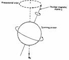
The nuclei of all elements carry a charge. When the spins of the protons and neutrons comprising these nuclei are not paired, the overall spin of the charged nucleus generates a magnetic dipole along the spin axis, and the intrinsic magnitude of this dipole is a fundamental nuclear property called the nuclear magnetic moment, µ. The symmetry of the charge distribution in the nucleus is a function of its internal structure and if this is spherical (i.e. analogous to the symmetry of a 1s hydrogen orbital), it is said to have a corresponding spin angular momentum number of I=1/2, of which examples are ¹H, ¹³C, ¹⁵N, ¹⁹F, ³¹P etc. Nuclei which have a non-spherical charge distribution (analogous to e.g. a hydrogen 3d orbital) have higher spin numbers (e.g. ¹⁰B, ¹⁴N etc).

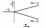
In quantum mechanical terms, the nuclear magnetic moment of a nucleus can align with an externally applied magnetic field of strength Bo in only 2I+1 ways, either re-inforcing or opposing Bo. The energetically preferred orientation has the magnetic moment aligned parallel with the applied field (spin +1/2) and is often given the notation a, whereas the higher energy anti-parallel orientation (spin -1/2) is referred to as b. The rotational axis of the spinning nucleus cannot be orientated exactly parallel (or anti-parallel) with the direction of the applied field Bo (defined in our coordinate system as about the z axis), but must precess about this field at an angle (for protons about 54°) with an angular velocity given by the expression:

w_o = gBo (1) (the Larmor frequency, in Hz)

The constant g is called the magnetogyric ratio and relates the magnetic moment m and the spin number I for any specific nucleus:

g = 2pm/hI (2) (h is Planck's constant)

For a single nucleus with I=1/2 and positive g, only one transition is possible (D I=1, a single quantum transition) between the two energy levels:

Energy levels at Ho

NMR is all about how to interpret such transitions in terms of chemical structure. We will first consider the energy of a typical NMR transition. If angular velocity is related to frequency by:

w_o = 2¼n, then n = gBo/2¼ (3)

It follows that proton NMR transitions (DI=1) have the following energy;

hn = DE = hgBo./2p (4)

For a proton g = 26.75 x 10⁷ rad T^-1 s^-1 and Bo ~ 2T, DE = 6 x 10^-26 J. The relative populations of the higher (n²) and lower (n¹) energy levels at room temperature are given by the Boltzmann law;

n²/n¹ = e-^DE/kT ~ 0.99999 (5)

For NMR, this means that the probability of observing a transition from n¹ to n² is only slightly greater than that for a downward transition, i.e. the overall probability of observing absorption of energy is quite small. This relationship also explains why a larger Bo favours sensitivity in NMR measurements, increasing as it does the difference between the two Boltzmann levels, and why NMR becomes more sensitive at lower temperatures.

Isotope:	^1H	^2H	^3H
Spin	1/2	1	1/2
Natural Abundance	99.985%	0.015%	---
Magnetogyric ratio (rad/T s)	26.7520 x 10^7	4.1066 x 10^7	28.535 x 10^7
Relative sensitivities	1.00	0.00000145	1.21
Magnetic Moment	4.83724	1.2126	5.1596
Quadrupolar Moment Q/m(2)	0	0.0028 x 10^28	0
Resonance Frequency	400 MHz	61.404 MHz	426.652 MHz

The situation for Other Nuclei

For other nuclei, the situation is much worse. Carbon has a resonant frequency range of 15000 Hz at typical values of Bo. Furthermore, equations (4) and (5) imply that not all nuclei are equally sensitive to the NMR experiment. Sensitivity is in fact proportional to g³, and since gc = 6.73 x 10⁷ rad T^-1s^-1, this makes carbon about 62 times less sensitive than protons. Since its spin active nucleus (¹³C) is only 1% abundant, the overall receptivity (= sensitivity times isotopic abundance) is 6200 times less and the scan width is 25 times greater than protons. To obtain a good CW type carbon spectrum might take 600 x 25 x 6200 s = 2.95 years. For ¹⁵N, this becomes 150 years!

Magnetic Properties of some useful Nuclei

Isotope	Natural Abundance %	Spin I=h/2p	NMR frequency MHz for 9.395 T	Relative sensitivity	Absolute sensitivity	Electric Quadrupole moment
^1H	99.980	½	400.000	1.00	1.00	-
^2H	0.015	1	61.402	9.65x10^-3	1.45x10^-6	0.227
^10B	19.580	3	42.986	1.99x10^-2	1.39x10^-3	11.1
^11B	80.420	3/2	128.335	0.17	0.13	3.55
^13C	1.108	½	100.577	1.59x10^-2	1.76x10^-4	-
^14N	99.630	1	28.894	1.01x10^-3	1.01x10^-3	2.0
^15N	0.370	½	40.531	1.04x10^-3	3.85x10^-6	-
^17O	0.037	5/2	54.227	2.91x10^-2	1.08x10^-5	-0.4
^19F	100.000	½	376.308	0.83	0.83	-
^27Al	100.000	5/2	104.229	0.21	0.21	14.9
^29Si	4.670	½	79.460	7.84x10^-3	3.69x10^-4	-
^31P	100.000	½	161.923	6.63x10^-2	6.63x10^-2	-
^33S	0.740	3/2	30.678	2.26x10^-3	1.72x10^-5	-6.4
^35Cl	75.500	3/2	39.193	4.70x10^-3	3.55x10^-3	-8.0
^37Cl	24.500	3/2	32.623	2.71x10^-3	6.63x10^-4	-6.2
^117Sn	7.610	½	142.501	4.52x10^-2	3.44x10^-3	-
^119Sn	8.580	½	149.089	5.18x10^-2	4.44x10^-3	-
^195Pt	33.800	½	85.996	9.94x10^-3	3.36x10^-3	-
^199Hg	16.840	½	71.309	5.67x10^-3	9.54x10^-4	-
^203Tl	29.500	½	228.597	0.18	5.51x10^-2	-
^205Tl	70.500	½	230.832	0.19	0.13	-
^207Pb	22.600	½	83.687	9.16x10^-3	2.07x10^-3	-

How to Detect all Frequencies Simultaneously.

Imagine the following thought experiment. Construct not one but two oscillators placed with their magnetic field along the x-axis in the diagram above, and two receivers detecting magnetisation along the y-axis. For protons, each would scan a different frequency range of 300Hz at 1Hz/second. The time taken to accumulate a spectrum would be halved from that for a single oscillator to 300 seconds. One could keep on adding oscillators until each would be required to scan a range similar to the actual width of the resonance being measured, for protons about 0.5Hz. Actually, 1200 such oscillators could have a fixed frequency, 0.5 Hz apart. The entire spectrum could be recorded by 1200 fixed frequency receivers in 600/1200 = 0.5 second!

It is of course not practical to design a spectrometer with 1200 oscillators each generating a fixed frequency. Lets go back to using a single oscillator (transmitter) and use this to generate a pulse of electromagnetic radiation of frequency w but with the pulse truncated after only a few complete cycles (corresponding to a duration t_p) so that the waveform has rectangular as well as sinusoidal characteristics. It can be proven that the frequencies contained within this pulse are within the range +/- 1/t_p of the main frequency w. For the proton example above, a pulse of 1/600 = 0.001667 seconds duration would generate a range of frequencies covering +/- 600 Hz, i.e. representing a typical chemical shift range at 60 MHz. For technical reasons, a shorter pulse covering a wider frequency range is often used.

A collection of Protons with different electronic environments spanning a range of 10 ppm at 60 MHz (600 Hz).

The "diamagnetic shielding" of the applied magnetic field by the electronic environment of each different nucleus in our collection produces slightly different local values of Bo and hence different characteristic Larmor frequencies for each unique nucleus.

B_eff = (1-s) Bo

where s describes the shielding of the effective magnetic field by the electrons surrounding the nucleus. The experiment described previously can be modified to detect nuclei resonating at different frequencies by making the transmitter sweep through the range of expected frequencies and recording the receiver response for each resonance. A machine built to such a specification is called a continuous wave or CW machine, such as one of the T-60 machines in the teaching laboratories. (Technically, it is actually easier to adjust Bo than +w on some machines, but that is a minor detail). However, a CW machine has one major disadvantage, which is that only one resonant frequency can be measured at any instant. For protons, the detected frequencies can differ by 600 Hz or more (at 60 MHz) and the time constants for relaxation described above limit the detectable response rate of the protons. In effect, this means that one cannot sweep through this frequency range at a rate of more than about 1Hz per second, i.e. it would take 600 seconds to record the spectrum.

Diamagnetic shielding: s_dia= 4pe²/3mc² r(r)/r dr

r(r)= electron density at a distance r from the nucleus, e = charge on the electron, m = electron mass and c = velocity of light.

Correlation of the chemical shift of the methyl group in CH₃X derivatives with the electronegativity of X

It can be seen that the shielding of the methyl protons is least in CH₃F where the highly electronegative fluorine atom strongly withdraws electron density from around the methyl protons. The induced currents in the halides have an additional influence over the shielding. This induced currents can better be seen in the following model.

Representation of ring currents in aromatic compounds.

Neighbor anistropic shielding effects are also produced by such group as

In the axially symmetric groups the component of magnetic susceptibility along the longitudinal axis of the bond (c_L) is very different to that along the transverse axis (c_T) and the contribution to the proton shielding is given by

s_anis= R^-3(1/3-cos³ q) (c_L -c_T)

In addition to diamagnetic shielding, a paramagnetic correction term s_para must be applied to allow for changes in the diamagnetic circulation occurring in atoms, which are part of a molecule, and not existing as free atoms. This may be thought as a distortion of the spherically symmetric environment of a free atom when it becomes part of a molecule. Its importance increases with the increasing atomic number of the nucleus.

s_para = -e²h²/m²c²<1/r³>_av 1/DE

where <1/r³>_av refers to the average distance of the 2p electrons from the nucleus and DE is an averaged electronic excitation energy.

There is also a correlation between the intramolecular electric field with chemical shift given by:

s_E = -AE_Z -B(E²+<E²>)

Where A and B are constants. E_Z is the component of the electric field acting along the bond. E² is the square of the total electric field at the nucleus, and <E²> is the time-averaged value of E².

Practical Aspects

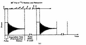
To obtain good spectra free from too much electronic noise, it is common to add together between 8 - 800 FIDs, a process which takes between ~30 seconds to 24 hours. Over that sort of period the field frequency may drift slightly, resulting in poor averaging. To compensate for this, most FT spectrometers have special "lock circuitry" based on detecting a deuterium signal. For this to work, the solvent used MUST contain deuterium! Normally CDCl₃ is used, but deuterated acetone or DMSO are also common, and "locking" the sample is normally the first operation actually performed on the spectrometer, and further the "lock signal" is also used to "shim" the spectrometer, i.e. adjust the homogeneity of Bo. Note that carbon tetrachloride should not be used as a solvent for this reason.

At the end of the short radio frequency pulse tp, the precession of all the nuclei in the magnetic field was effectively in phase. Provided measurement of the resultant induced signal in the y-axis starts immediately afterwards, all the initial measured sine wave responses would also be in phase. However, no NMR spectrometer yet constructed can achieve this and for electronic reasons, a short delay between the end of t_p and start of measurement is required. The short delay means measurement begins when the sine waves are already out of phase. This so called first order phase error can be calculated from a suitable combination of the real and imaginary components of F(w). Another phasing error due to technical imperfections in the spectrometer is often referred to as the zero order phase correction. These are both applied to F(w) after the FT is complete.

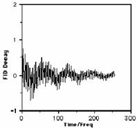
With the measurement of a single FID resulting from one pulse, followed by Fourier Transformation to give F(w), one can achieve a spectrum approximately equivalent in its noise level to a CW spectrum which took 600 or more seconds to record! By adding n FID measurements together in the computer, one can reduce the noise by ˆⁿ, i.e. 64 FIDs added together (and taking 3.41*64= 3.6 minutes) will reduce the noise by almost a factor of 10. It also turns out that one can multiply the whole of f(t) by a new function such as a decaying exponential prior to the FT operation. Surprisingly, this does NOT introduce any new frequencies, but can dramatically reduce the noise level at the expense of making the resulting peaks broader. This is because a faster f(t) decay corresponds to a shorter relaxation time T, a larger 1/T, and hence wider peaks (c.f. ¹⁴N).

Other more complex functions (weighting functions) can actually decrease apparent peak width, this time at the expense of the noise level. The effects of such functions, as well as first order phase and non-Nyquist sampling errors etc are readily demonstrated using a relatively short computer program. Such a program is in fact described as one of the Fortran programming course projects, the output of which is shown below;

Summary

We have set out how a short pulse of electromagnetic radio frequency radiation can establish a resonance with precessing nuclei in an applied magnetic field, and in doing so establish a coherent phased precession which effectively tilts the precessing magnetisation vector away from the axis of the applied field by a certain angle called the pulse angle. This induces a response in a detector, which is measured as a function of time and can be converted to a more readily interpreted frequency domain signal by digitisation and Fourier Transformation. A whole range of more sophisticated experiments can be derived from this simple one by varying the pulse angle, adding extra pulses and inserting time delays, the entire assemblage being called a pulse sequence.

The Pulsed NMR Experiment

Let's go back to our Precession Diagram. Our transmitter oscillator placed perpendicular to B_o generates a pulse of electromagnetic radiation producing a magnetic field B1 along the x-axis. A range of frequencies +w ± 1/t_p are produced, enabling resonance to be simultaneously established with all the Larmor frequencies of protons within 1/t_p of +w. The phase of each set of identical resonances is rendered coherent, which "tips" the macroscopic magnetisation vector for each resonance away from Bo, by the angle q defined by:

q = g. B1.t_p (6)

A value of q =90° is often referred to as a 90° pulse because of the angle the magnetisation vector is changed by, i.e. from the z axis into the xy plane! In practice, values of q ~30° are often selected for practical reasons, although even 180° pulses are sometimes used.

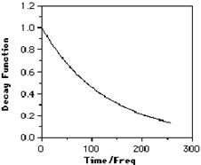
Our particular pulse stops after tp seconds, when all the various protons have an excited state population which is no longer in equilibrium with the ground state as defined by equation (5) (indeed as noted above, with a 180° pulse the equilibrium is inverted). Equilibrium is re-established via spin-lattice and spin-spin relaxation, a process which takes about 5-6 seconds for protons (c.f. T₁and T ₂ above) and which involves the return of the macroscopic vector M to the z axis, i.e. the "flip" angle q decays back to zero (exponentially) in about 5-6 seconds for typical protons. M for each set of different protons will have a different Larmor precession frequency, which in this example will span the range 600 Hz. As long as q is not 0, the resultant non-zero vector component of M in the direction of the receiver coil placed on the y-axis induces a sinusoidal current in this receiver. Each set of distinct protons will produce a sine (or cosine) wave whose frequency matches their precession frequency and the intensity of which is related not only to the phase of the sine wave but also to the value of q at any instant (i.e. the magnitude of the y component of M). The signal detected in the receiver therefore resembles a collection of exponentially decaying sine waves, and is called a Free Induction Decay, or FID for short;

For practical reasons, electronic circuitry in the receiver automatically subtracts the transmitter frequency +w from the measured frequencies so that only frequencies in the range 0 - 600 Hz are actually recorded. You should also note that in discussing the behaviour of the vector M, our reference point was the so called "laboratory frame of reference" in which M is "observed" to precess with frequency +w. We will simply note here that it is actually more convenient to refer to a "rotating frame of reference" in which the "observer" is assumed to be also rotating around at +w (rather like riding on a carousel rather than watching it from afar) which makes the vector M appear stationary. Such descriptions are used when describing more complex NMR experiments (i.e. two-dimensional NMR) but will not be discussed further in this particular course.

Relaxation

Once the magnetization has been excited with a pulse, it needs to return to equilibrium. The process that returns the magnetization to the +Z axis is called the Spin-Lattice relaxation time and is abbreviated: T ₁ (do not mix this term with the evolution time t1 in 2D NMR.

Once the magnetization is coherent in phase in the XY plane (transverse plane) after a pulse,
it needs to return to equilibrium: by loosing it's phase coherence. This relaxation time is called the Spin-Spin relaxation time and is abbreviated: T₂ (do not mix this term with the acquisition time t2 in 2D NMR).

This process can be best measured with the Spin Echo experiment. This experiment can also be used to measure diffusion in the NMR tube by using gradients.

Spin-lattice Relaxation time T₁ (longitudinal)

The relaxation time T₁ represents the "lifetime" of the first order rate process that returns the Magnetization to the Boltzman equilibrium along the +Z axis. T₁ relaxation time can be measured by various techniques described in the table below.

Name	Pulse Sequence	Signal evolution vs T1
Inversion Recovery (IRFT)	D1-180-tau-90-Acq {D1+Acq>5*T1}	M (tau)/M0= 1-2*exp(-tau/T1)
Progressive Saturation (PSFT)	(dummy pulses)-D1-90-Acq {tau=D1+Acq}	M (tau)/M0= 1-exp(-tau/T1)
Saturating Comb (Mainly useful in solid) require: T2*<<T1	{n*90-t}-tau-90-Acq t: pulse spacing during Comb. :T2*< t <T1 tau: delay for magnetization recovery	M(tau)/M0= 1-exp(-tau/T1)

After a delay of 1*T₁, 63% of the magnetization is recovered along the +Z axis. To recover 99% of the magnetization a delay of 5*T₁ need to be used.

The magnitude of the relaxation time depends highly on the type of nuclei (nuclei with spin 1/2 and low magnetogyric ratio have usually long relaxation time whereas nuclei with spin>1/2 have very short relaxation time) and on other factors like the physical state (solid or liquid state), on the viscosity of the solution, the temperature ... etc. in other words the relaxation time depends on the motion of the molecule.

The longitudinal relaxation process (T₁) governs the time interval between 2 transients.

· If the interval between 2 transients is shorter than 5*T₁, the accuracy of the integration might be questionable.

· If the interval between 2 pulses is shorter than 5*T₁, as for obtaining routine NMR spectra, the pulse width must be adjusted to accommodate the different length of the relaxation process to obtain the best sensitivity for the NMR experiment.

· The length of the pulse that provides the best sensitivity for a given relaxation time is called the "Ernst angle". For example: if 1-sec. acquisition time is used, you can find below the best pulse angle to use for different relaxation time.

Relaxation time (sec)	Ernst Angle (with 1 sec repetition time)
100 (very slow T1)	8 degree
10	25 degree
4	33 degree
2	53 degree
1	68 degree
0.4	86 degree
0.1 (rapid T1)	90 degree

Relaxation and Molecular Motion

The relaxation process is induced by field fluctuation due to molecular motion. (The local field experienced by a molecule changes when the molecule reorients)

A few definitions:

The correlation time -tc (Tau-c): represents the time it takes for a molecule to reorient by 1 degree ("tumbling time").

The spectral density - J(w): describes the ranges of frequency motion that are present. Not all molecules tumbles at a unique rate: molecules tumbles, collide, change direction... at a range of rates up to the maximum rate of (1/tc). The concentration (or intensity) of fields at a given frequency of motion (w) is known as the spectral density J(w).

There are several relaxation mechanisms:

Interaction	Range of interaction (Hz)	Relevant parameters
1- Dipolar coupling	10^4 - 10^5	- Abundance of magnetically active nuclei - size of the magnetogyric ratio
2- Quadrupolar coupling	10^6 - 10^9	- Size of quadrupolar coupling constant - electric field gradient at the nucleus
3- Paramagnetic	10^7 -10^8	Concentration of paramagnetic impurities
4- Scalar coupling	10 - 10^3	Size of the scalar coupling constants
5-Chemical Shift Anisotropy (CSA)	10 - 10^4	- Size of the chemical shift anisotropy - symmetry at the nuclear site
6- Spin rotation

All of them (except scalar mechanism) involve the magnetogyric ratio of the nucleus. The first 3 mechanisms are much stronger and efficient than the other 3 mechanisms.

There are different approaches to distinguish the various relaxation mechanisms:

1. By the strength of the interaction

2. By the use of isotopic substitution to identify the dipolar mechanism

3. By the field dependence: CSA is proportional the Bo (applied field). Quadrupole interaction is inversely proportional the Bo (applied field)

4. By their temperature dependence

You will find below a very brief description of those mechanisms. In general terms, the relaxation rate R₁ (1/T₁) depends on the strength of the interaction and on a correlation function.

1- Dipole-Dipole interaction "through space"

This relaxation mechanism is particularly important for molecules containing protons (high natural abundance nuclei equipped with a large magnetogyric ratio).

This interaction depends on the strength of the dipolar coupling (depends on gamma), on the orientation/distance between the interacting nuclei and on the motion.

R₁ = k * g₁² * g_S² *(r1s) ^-6 * t_c

· The distance dependence is very large as can be seen in Carbon-13 (protonated carbons relax more rapidly than quaternary)

· The dependence on gamma is also very large. Proton relaxation is dominated by dipolar relaxation. X-H (hetero nuclei directly substituted by proton) is also dominated usually by dipolar relaxation due to the short distance and due to the fact that proton has a strong gamma-ratio. If proton is replaced by deuterium, in the X-D bond, the X-nuclei relax much slower than the corresponding X-H due to the lack of dipole-dipole relaxation. (Gamma-H is 6.5 time larger than gamma-D).

2- Electric Quadrupolar Relaxation

If a nuclei has a spin>1/2, it is characterized by a non-spherical distribution of electrical charges and possesses an electric magnetic moment. The quadrupole coupling constant is in the MHz range (very efficient). As this relaxation process is very large, it dominates over the other mechanisms.

This relaxation depends on:

1. "eQ" - the quadrupole Moment of the nucleus e.g. Deuterium: eQ=.003 and ⁵⁵Mn has eQ=0.55

2. "eq" - the Electric Field Gradient (EFG).

The Quadrupole coupling vanish in a symmetrical environment. e.g. for symmetrical [NH₄}⁺ : eq * eQ = 0 and therefore has very long T₁ =50 sec, whereas CH₃CN : eq * eQ about 4 MHz and T₁=22 msec.

3- Paramagnetic Relaxation

The molecular motion modulates the electric field from unpaired electron spin.

· There is dipole relaxation by the electron magnetic moment.

· There is also a transfer of unpaired electron density to the relaxing nucleus.

4- Scalar Relaxation (due to coupling with fast relaxing quadrupolar nuclei)

The effect of scalar coupling relaxation on T₁ is significant only if the two interacting nuclei have very close frequency. This condition occurs very rarely!

It occur for example for Carbon-13 (75.56 MHz with B1=7.06 T) and Br-79 (75.29 MHz with B1=7.06 T) which are very close in frequency.

Scalar relaxation is more important for the T₂ relaxation as with this mechanism the quadrupolar nuclei can broaden lines significantly on nuclei that are coupled to it.

5- Chemical Shift Anisotropy Relaxation

The magnetic field sense by the nucleus depends on the chemical shift tensor in the molecule.

The chemical shift is in fact dependent by the orientation of the molecule in the magnetic field. This effect, called the chemical shift anisotropy (CSA), is very well known in solid state NMR as it is responsible (in part) for the very wide line width observed on a static sample.

In solution, CSA is averaged out by molecular tumbling and a sharp isotropic shift is observed; but the modulation of the shielding can provide a relaxation mechanism in absence of other mechanism. This mechanism is field dependent.

CSA is an important relaxation mechanism for nuclei with large chemical shift scale as for example on Phosphorus-31 and on Cadmium-113.

6- Spin Rotation

Intramolecular dynamic process (like the rotation of methyl group) can also contribute to longitudinal relaxation.

Spin-Spin Relaxation time T₂ (transverse)

The existence of relaxation implies that an NMR line must have a width. The smallest width can be estimated from the uncertainty principle. Since the average lifetime of the upper state cannot exceed T₁, this energy level must be broadened to the extent: h/T₁. This means that line width at half-height of the NMR line must be at least: 1/T₁.

In Solution NMR, very often T₂ and T₁ are equal (small/medium molecules and fast tumbling rate). For solids, T₁ is usually much larger than T₂. The very fast spin-spin relaxation time provides very broad signals.

There are other processes that can increase the line width substantially over the expected value extracted from T₁ analysis. T₂ represents the lifetime of the signal in the transverse plane (XY plane) and it is this relaxation time that is responsible for the line width. The "true" line width on an NMR signal depends on the relaxation time T₂ (line width at half-height=1/T₂).

In fact, by measuring the experimental line width, one can in principle determine the T₂ relaxation time. Unfortunately, the experimental line width depends also on the inhomogeneity from the magnetic field. The experimental relaxation time, extracted from the line width, is called T₂*(T₂*=T₂+T₂ (inhomogeneity)). The inhomogeneity factor is more critical for nuclei with higher frequency (more critical for proton than for Carbon or Phosphorus). The reason behind this statement can be explained as follows: imagine that identical nuclei (identical chemical shift) in a NMR tube are submitted to slightly different field (inhomogeneity from the magnet). The resonance frequency for each individual nucleus is described by the equation: n=gB_o. If the field vary through the NMR tube, so do the observed frequency, broadening the NMR line. This broadening would affect more the proton (higher g) than lower frequency nuclei. The broadening is in fact directly proportional to the frequency.

Spin-Spin relaxation mechanisms

The same mechanisms that are active in Spin-Lattice are active for spin-spin relaxation. We will describe here the mechanisms that can bring extra broadening to the peak.

Scalar relaxation (dynamic NMR and scalar coupling with quadrupolar nuclei)

Scalar relaxation occurs when two spins interact through bond (electron mediated) - J coupling.

Spin I can feel fluctuating in the field from spin S in two ways:

1. The scalar coupling J can be time dependent due to chemical exchange, If nuclei S is jumping in and out of a site in which it is coupled to spin I, splitting will collapse at high rate. At intermediate rate, the line will broaden due to partial scalar coupling (this can be observed on exchangeable protons like OH or NH)

2. The spin S can be time dependent due to rapid relaxation of spin S (like in quadrupolar nuclei)

Relaxation induced by Quadrupolar nuclei

If the relaxation time of the quadrupolar nuclei is rapid (1/T₁(S) >> 2pJ), nuclei I will not couple to the quadrupolar nuclei. e.g. ¹H next to ¹⁴N or ¹¹B (T₁ => 10-100 msec) => produce broadened lines, e.g. ¹H next to ³⁵Cl (T₁ => 1 usec) => insignificant broadening.

Scalar coupling with rapidly relaxing quadrupolar nucleus can be determined based on T₁ and T₂ analysis.

Measurement of T₂ relaxation process

In non-viscous liquids, usually T₂ = T₁. But some process like scalar coupling with quadrupolar nuclei, chemical exchange, interaction with a paramagnetic center, can accelerate the T₂ relaxation such that T₂ becomes shorter than T₁.

In principle T₂ can be obtained by measuring the signal width at half-height (line-width = (pT₂)^-1

However the line width for non-viscous liquids is most often dominated by field inhomogeneity. Fortunately, the dephasing of spins isochromats resulting from field inhomogeneity is a reversible process: it can be refocused by using a 180 degree pulse inserted in the center of an evolution time.

Processing the Free Induction Decay.

We now have a signal corresponding to our NMR spectrum which contains a set of sine/cosine waves measured as a function of time and decaying towards zero intensity at an exponential rate (or more accurately to an intensity indistinguishable from the electronic noise in the receiver). This signal is said to be analogue, i.e. it varies continuously with time and is described as a time domain signal. There is little point in recording this on a chart recorder, since its complexity would make it unintelligible. Instead, it will be stored on computer memory, and to achieve this it needs to be digitised. This is done by sampling the intensity of the signal at discreet time intervals using a device known as an ADC (Analogue-to-Digital-Convertor) and storing the intensity as an integer value ranging from 0 to e.g. 2²⁴ (on cheaper spectrometers, only 2¹⁶!)

Two questions must now be answered; how frequently does one sample the FID, and for how long? The answer lies in the Nyquist Theorem, which states that to define a full (2p) cycle of a sine wave, its intensity must be sampled at least twice during one cycle. We need to sample at intervals which will therefore allow the highest frequency sine wave to be sampled, which in the example set out above is actually 600 Hz. Sampling must therefore occur every 1/2*600 = 0.0008333 seconds. For how long? Well, to avoid losing information, our digital spectrum must eventually be able to distinguish between two peaks in the NMR spectrum say 0.293 Hz apart, similar in magnitude to the smallest couplings normally seen in standard samples, and referred to as the required digital resolution of the spectrum. This actually needs 2048 digital points in a spectrum that will be eventually 600 Hz wide (600/2048 = 0.293). Why did we pick exactly 0.293 Hz and hence require exactly 2048 points? Because all this digital information is going to be processed using a mathematical technique known as Fourier Transformation (FT), and FTs are particularly fast (i.e. they are FFTs) when the number of points processed is exactly 2ⁿ (n is an even integer, in this case 10);

F(w) = f(t) e^-iwtdt (5)

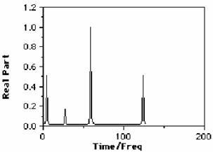
Here, the FID = f(t), and F(w) is the same data expressed as frequencies (=1/T) rather than as times and is called a frequency domain spectrum. This is the form we know for "conventional" NMR spectra, i.e. frequencies relative to an internal standard such as TMS. Equation (5) cannot be integrated analytically, and numerical methods such as the Cooley-Tukey algorithm have to be applied. The right hand side of equation (5) can also be expressed as;

F(w) = f(t) cos -wt + f(t)i sin -wt (6)

which means that F(w) has two components, referred to as the real and imaginary parts. Each component contains the same frequency data but with a different combination of phase and amplitude. Only the real component is normally displayed. For 2*2ⁿ points in f(t), only 2ⁿ unique frequencies in F(w) are obtained. The total number of points to be measured therefore to achieve an eventual resolution of 0.293Hz over a width of 600 Hz actually corresponds to 2 * 600/0.293 = 4096 points, and our total sampling time is 4096 * 0.0008333 = 3.41 seconds. At the end of this time, the time constants defining the exponential decay of q means it is normally close to zero, f(t) is effectively zero and the entire cycle can start again with a new pulse. Finally, we note that the time constants involved in the exponential decay of q (T1 and T2) are manifested in the Fourier Transformed function F(w) via 1/T, which has the same unit (Hz) used to measure the width of a NMR peak. Put another way, if M did not decay at all, T1 = T2 = ƒ and F(w) would have infinitely narrow and hence lead to unobservable lines, i.e. 1/ƒ = 0 Hz. This also explains why it is not a good idea to clean NMR tubes with chromic acid. Traces of this (paramagnetic) substance provide an excellent mechanism for M to relax, T1 ~ 0, and hence the peaks are infinitely wide, i.e. also unobservable.

Applications of ¹H NMR

In contrast to carbon, proton spectra tend to be much more complicated in appearance due to a) the smaller chemical shift range found for typical compounds (~ 20 ppm at most) and the wide variation in the magnitude of the coupling constants. You should by now be aware of typical chemical shift values found for protons:

H-C-C, 0-2 ppm; H-C-C=O, ~2 ppm; H-C-N, ~3 ppm; H-C-O, ~4 ppm; H-C=C, ~5 ppm; H-aromatic, 6-7 ppm; H-C=O, ~9 ppm; H-O-C=O, ~12 ppm (for more extensive tables, see the recommended text).

This information supplements that obtainable from ¹³C spectra. We will focus on the type of information not obtainable from ¹³C spectra, namely stereochemical information derived from the numerical values of coupling constants and the techniques used to derive this information.

Homonuclear coupling

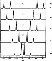
As noted above, the coupling J is a manifestation of the splitting of Bo by the essentially equal populations of the ground and excited energy levels of a spin 1/2 nucleus. As such, it depends not on the absolute value of Bo but on the characteristics of the nuclei involved and in particular of the bonding electrons between them. Chemical shifts on the other hand are directly related to relative Larmor frequencies, and so do depend on Bo. Let us illustrate this with part of the spectrum of trans3-phenyl propenoic acid, which gives rise to a so-called two-spin system. The spin system is referred to as AB if the chemical shifts are quite close together, and AX if they are far apart.

The spectra are shown at different values of Bo, corresponding to Larmor proton frequencies of wo=60, 100, 300 and 600 MHz (the practical limit for a spectrometer is around 1000 MHz, of which only one is currently installed, in the United States). Each proton signal is split into two by the presence of the other (2nI+1, n=1, I=1/2), the splitting being given by J = d * w/10⁶, which in each spectrum is approximately 16 Hz. Before we discuss the chemical interpretation of this value, we note that a) the 600 MHz spectrum appears simpler than the 60 MHz version and b) the 60 MHz relative peak intensities are dramatically different from those at 600 MHz. As J (in Hz) becomes numerically similar to the difference in Larmor frequencies (in Hz) between the two protons (Dwo = d * w_average/10 ⁶) the spectra are said to become more "second order", the prime manifestation of which is the "tilting" of the intensities of each doublet towards the other.

J = [L₁-L₂] = [L₃-L₄]

If (ua-ub)²>J² ® ua = (L₁+L₂)/2 and ub = (L₃+L₄)/2

L₁-L₃ = [(ua-ub)²+ J²]^1/2 = 2C

L₂+L₃ = ua+ub ® ub = {L₂+L₃-(L₁-L₃)²-J²]^1/2}/2

ua = L₂+L₃- ub

(ua-ub) = (4C²-J²)^1/2 ® [(2C-J) (2C+J)]^1/2

dab = (ua-ub) = [(L₂-L₃)(L₁-L₄)]^1/2

Line	Frequency	Relative Intensity
L1	C+1/2 J	1-J/2C
L2	C-1/2 J	1+J/2C
L3	-C+1/2 J	1+J/2C
L4	-C-1/2 J	1-J/2C

If ua = ub then,

E₁ = ua + J/4; E₂ = J/4; E₃ = - J/4; E₁ = -ua + J/4

L₂ = L₃ ® ua

L₁ = L₄ = 0

Spin System

Spin	System	# of Lines	Intensity	Example
2	AB	4	See above
2	AX	4	~ 1:1	CHFCl2
3	AB2	8+1	da=L3 db=(L5+L7)/2 JAB= (L1-L4+L6 -L8) /3 The intensities depend on the J/d ratio
3	ABC	12+3	f8= bbb E = -3/2 f6= bab f6= bab f7= abb E = -1/2 f2= aab f3= aba f4= bba E = 1/2 f1= aaa E = 3/2 DE= ± 1 ® 15 allowed transitions
3	ABX	12+2	Discussed in the text
3	AMX	12	May be considered as three double of doublet
3	AX2	5	1:2:1	CHF2Br
4	A2B2	14+4+2	Complex	Very few examples SF4 at -100°C
4	A2X2	6	1:2:1	CF2=C=CH2
4	AA'BB'	24	Complex
4	AA'BB'	24	Complex
4	AA'XX'	20	Complex
4	AB2X	18+4	Complex
4	AB3	14+2	Complex
4	ABC2	28+6	Complex
4	ABCD	32+24	Complex
4	ABCX	32+18	Complex
4	ABX2	18+4	Complex
4	AX3	6	~ 1:3:3:1 ~1:1	^13CH3Cl
5	A2B2C	78	Complex
5	A2B3	25+9	Complex	PhSCH2CH3
5	A2BCD	128	Complex
5	A2X3	7	~1:3:3:1 ~ 1:2:1	ClCH2CF3
5	A3BC	61	Complex
5	AA'BB'X	64	Complex
5	ABCDE	210	Complex
5	AMX3	20	Complex	^13CH3F
6	A2B2C2	180	Complex
6	A2B2CD	296	Complex
6	A3B3	68	Complex	^12CH3^13CH3
6	ABCDEF	792	Complex
6	ABCR3	109	Complex
6	ABXR3		Complex

Since J coupling depends on the intervening bonds and electrons, its value is highly characteristic of these bonds. In this case the coupling arises from three intervening bonds, and hence we term it ³J_H-H coupling.

The coupling mechanism for ¹³C-¹H can be visualized as follows:

¹³C e¯ e ¯¹H

which gives a positive coupling, while for coupling over more than one bond, the mechanism of transmission via the intervening atoms is less direct and, in consequence, both positive and negative coupling are found.

The value depends one the dihedral angle between the two C-H bonds by the expression:

J_(HC-CH) = 10 cos² f

For the system: H-C-H: J = -10 to -18 Hz.

¹H ¯ e e¯ ¹³C e¯ e ¯¹H

ABX spin system

Here three different protons all couple to one another (described as an ABX spin system), and the 2nI+1 rule must be applied in stages as follows;

Each proton is described as a double doublet, since the two couplings involved are numerically different. The actual values when measured from the spectrum are; da 2.72, db 3.25, dc 4.38 ppm; J_ab = 18 Hz, J_ac = 2, J_bc = 10 Hz.

For the ABX system:

Origin Energy Intensity B 1/2(ua+ub)-1/2(Jab+N)-D- 1-sin f- B 1/2(ua+ub)-1/2(Jab-N)-D+ 1-sin f+ B 1/2(ua+ub)+1/2(Jab-N)-D- 1+sin f- B 1/2(ua+ub)+1/2(Jab+N)-D+ 1+sin f+ A 1/2(ua+ub)-1/2(Jab+N)+D- 1+sin f- A 1/2(ua+ub)-1/2(Jab+N)+D- 1+sin f- A 1/2(ua+ub)-1/2(Jab-N)+D- 1+sin f+ A 1/2(ua+ub)+1/2(Jab-N)+D- 1-sin f- A 1/2(ua+ub)+1/2(Jab+N)+D+ 1-sin f+ X ux-N 1 X ux+D+-N- ½[1+cos(f+-f-)] X ux-D++N- ½[1+cos(f+-f-)] X ux+N 1 Comb ua+ub-ux 0 Comb ux-D+-D- ½[1+cos(f+-f-)] Comb ux-D++D- ½[1+cos(f+-f-)]

D±cos f±=½(dab±L) and D±sin f±=½(Jab) Þ D±=½[(dab±L)^2+J^2ab]^½ N=½(Jax+Jbx) L=½(Jax-Jbx) For a (+½) X orientation, the effective d will be u^*a=ua+½Jax u^*b=ub+½Jbx dab = ua-ub d^*ab= dab +½(Jax-Jbx)= dab+L Mid.pt =½(ua+ub)+1/4(Jax+Jbx)=½( ua+ub)+½N=[(F8-F2)(F6-F4)]^½ and for b (-½) X orientation, the value are u^*a=ua+½Jax u^*b=ub+½Jbx d^*ab= dab -½(Jax-Jbx)= dab-L Mid.pt =½(ua+ub)+1/4(Jax+Jbx)=½( ua+ub)-½N Jab=F3-F1=F4-F2=F7-F5=F8-F6 Jax+Jbx=F12-F9 F4-F3=F2-F1=F12-F10=F11-F9 F8-F7=F6-F5=F12-F11=F10-F9

Subspectra 1=(94.6+79.3+72+56.4)/4=75.6

Subspectra 2=(98.9+83.7+80.4+64.7)/4=81.9

Center= (75.6+81.9)/2=78.75

d_ab=½{[(F₇-F₁)(F₅-F₃)]^½+ [(F₈-F₂)(F₆-F₄)]^½}=½(16.7+10.6)=13.7

u_a=center+½ d_ab=78.75+6.85=85.6 Hz (solid line)

u_b=center-½ d_ab=78.75-6.85=71.9 Hz (dotted line)

u_x= 183.2 Hz

J_ab= 15.4 Hz, J_bx= 9.4 Hz, J_ax= 3.4 Hz.

In cases where homonuclear coupling occur, the Hahn echo sequence will not refocus the homonuclear scalar coupling, as the 180 degree pulse is inverting both nuclei at the same time. This double inversion gives rise to what is known as "J-modulation".

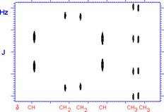
The measurement of the spectra by incrementing systematically the tau delay, yield to 2DJ NMR where only the scalar coupling evolves as a function of the whole spectra.

Other Types of Coupling

⁴J for allylic coupling, H-C=C-C-H varies from -3 to +2 Hz, depending again on the angle between the two H-C bonds. In aromatic systems, ³J or ortho coupling ~ 7-8; ⁴J or meta coupling ~ 2 Hz; ⁵J or para coupling ~ 0.5 Hz. Large long range coupling is not often observed, but one type of system does reveal a dramatic dependence on geometry, often called "W" coupling because of the relationship between the two protons:

For alkenes the couplings are:

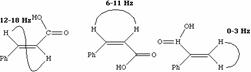
The last example is actually a ²J coupling at a sp² carbon.

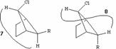
Whereas in the alkene example previously only two angles between the H-C bonds are possible, here values ranging from 0 - 180 ^* may occur. A theoretical relationship describing the value of J in terms of the angle between the two bonds involved in such ³J coupling was derived by Karplus.

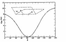
From this one can immediately conclude that J_ac must correspond to a gauche coupling (~60š) and J_bc to an anti coupling (~180š). Note also that at about 90š, J~0 a situation often encountered in many molecules. The largest coupling of +/-18 Hz is typical of the two bond ²J H-C-H system (compare that with the ²J H-C-H coupling in alkenes, where J is close to zero), and from other experiments can actually be shown to be negative! The NMR data therefore allows the conformation shown above to be proposed, and illustrates the powerful utility of NMR in such conformational analysis.

Before we leave this system, we ask why the ²J H-C-H coupling in this compound is visible, whereas that in e.g. bromoethane is not. If a CH2 group is close to a chiral center in the molecule, the two methylene protons are said to be diastereotopic and are likely to have differing chemical shifts and different coupling to adjacent protons. This effect arises NOT from any restricted rotation about the C-C single bond, but from the absence of any possible plane of symmetry bisecting the methylene group. As can be seen from the Newman projection above, in all possible conformations for this molecule, Ha and Hb are always in a different environment; this would not be true of e.g. bromoethane.

Heteronuclear coupling: Coupling Between Protons and Other Nuclei.

We have seen previously how ¹H- ¹³C coupling can help in understanding ¹³C spectra but such coupling is not apparently observed in ¹H (thank goodness) because on average there is only a 1% probability that a given proton will be adjacent to a ¹³C nucleus. However, if you look about ²J_H-C 2 ~ 65 Hz away from a strong proton peak (e.g. methanol) you may see a small peak about 0.5% of the intensity of the central proton peak. This is the so-called carbon satellite arising from just such hetero-nuclear coupling. Observing such satellites can sometimes have uses. Another satellite due to ²J_Si-CH coupling is often observed (but rarely correctly attributed) as a small peak +/-3 Hz of the proton TMS signal and about 2.5% the height. Satellites are commonly observed in spectra of many other elements where the isotopic abundance is not 100%.

Finally if either ¹⁹F or ³¹P are present in a molecule, both are likely to couple to protons since these isotopes are 100% abundant. Typical couplings are ¹J_H-P ~ 200-700 Hz, ²J_HC-P ~ 0.5 - 20 Hz; ²J_HC-F ~ 45 Hz, ³J_HC-F ~ 5-20 Hz.

Simplification of Spectra

The three spin proton system discussed above had 12 lines, but even so the "tilting" and closeness of the peaks frequently results in spectra that are very difficult to interpret. Many modern techniques are available for dealing with this problem. Here we will deal with only a few to give some flavour of how these problems are approached.

Use of Higher Fields

We saw in the spectra of trans-3-phenyl propenoic acid how high field can "stretch" out the spectrum, such that each distinct proton is revealed as a separate multiplet. The current limit corresponds to 1000 MHz. Such spectrometers are ultra-expensive, and not available to all.

Homonuclear Decoupling

This technique was mentioned in the context of carbon NMR, where all the protons were decoupled from the carbons to achieve a simplified ¹³C spectrum. Similarly, if a strong electromagnetic field (the "decoupler") is applied at exactly the resonant Larmor frequency of one proton in a compound, that specific proton apparently loses its entire coupling to other protons and if you are lucky, the spectrum is simplified.

Our second example of decoupling also introduces the concept of a "difference spectrum". If a spectrum is recorded twice, once with the decoupler on and once with it off and the two spectra are subtracted, what remains (in principle) is the effect due to decoupling

Intensity Measurements

The strength of an NMR signal, which is measured by the area under the NMR line, is proportional to the number of nuclei contributing to the line. Accurate measurements of these areas greatly facilitate the interpretation of spectra and also provide a means of conducting quantitative analyses. Such integrations can be accurate to within 1-2% provided signal/noise is sufficiently high.

Dynamic Processes

Whenever a molecule contains exchangeable proton such as COOH, OH, NH, NH₂, then several spectral possibilities may be seen depending upon whether the proton exchange rapidly, slowly or not at all with themselves or with other parts of the system (H₃O⁺, OH^- or H₂O), a good examples provided by the spectrum of purified ethanol.

Dynamic processes may be divided into two main types:

a) Intermolecular effects which include electron transfer, exchanging groups, hydrogen bonding, molecular association and ion solvation.

b) Intermolecular exchange includes conformational interconversion in cyclic systems, rotation about single bonds, and atom inversion.

Slow Exchange: If the exchange process taking place between two species is very slow compared with the magnetic resonance detection process, then a distinct signal will be observed for each species. The keto-enol equilibrium of acetylacetone at room temperature shows an example of this type of behaviour.

Fast exchange: Hydrogen bonding provides the best example of very fast exchange where only one absorption band is observed. The nuclear magnetic resonance experiment detects a band (u) corresponding to the weighted mean of two signals of the bonded hydrogen and the more shielded non-bonded species

u = p₁ u₁ +p_n u_n

Where u, u₁, and u₂, are the observed frequency, the pure monomer frequency, and the pure n-mer (aggregate) frequency respectively. p₁, and p₂ are the population fractions of monomer and n-mer.

Medium Effects on Chemical Shifts

The total effect of the solvent on nuclear shielding is given by:

s _(solvent) = s_B+ s_W + s_A + s_E + s_H

s_B = Bulk magnetic susceptibility of the medium. Depends on the external reference.

s_W = Effect of the weak van der Waals forces between solute and solvent. Such effect can distort and change the symmetry of the electronic environment a given nucleus. Generally, large polarizable halogen atoms in the solvent leads to increased negative values of s_{W .}

s_A = Magnetic anisotropy in the solvent molecules and arises from the nonzero orientational averaging of solvent with respect to solute.

s_E = The effect of electric field on nuclear shielding. When a polar molecule is dissolved in a dielectric medium, it induces a reduction in the shielding around a proton in the solute.

s_H = A specific solute-solvent interaction, the mast important of which is hydrogen bonding.

Solvent Effects on Coupling Constants

While Solvent effects on chemical shifts can be quite large, the effect of solvent on coupling constant is usually small, 1-2 Hz for geminal H-H coupling.

Solvent effects on Relaxation and Exchange Rates

T1 and T2 depend on the rate of molecular tumbling, which in turn, is a function of the viscosity of the solvent, so that, an increase in viscosity reduces the relaxation times and thus broadens the resonance lines. DMSO is a very viscous solvent, at room temperature lines of compounds dissolved in this solvent are broader than in other solvents

Hydrogen Bonding

Proton chemical shifts are extremely sensitive to hydrogen bonding. In almost all cases, formation of a hydrogen bonding causes the resonances of the bonded proton to move downfield by as much as 10 ppm.

Effect of Paramagnetic Species

Mettalo-oragnic compounds in which the metal is diamagnetic display chemical shifts for proton resonance that cover only a slightly larger than that found for organic molecules. If the metal is paramagnetic, chemical shifts for protons often cover a range of 200 ppm, and for other nuclei the range can be greater. These large chemical shifts arise from either a contact interaction or pseudocontact interaction. The former involves the transfer of some unpaired electron density from the metal to the ligand.

The pseudocontact interaction (dipolar interaction) arises from the magnetic dipolar fields experienced by a nucleus near a paramagnetic ion. The effect is entirely analogous to the magnetic anisotropy.

Both contact and dipolar shifts from unpaired electrons are temperature dependent, normally varying approximately as 1/T. The presence of unpaired electrons usually causes rapid nuclear relaxation and leads to line broadening.

Lanthanide Shift Reagents

The large chemical shift caused by paramagnetic species have been exploited in shift reagents, The object is to induce large alterations in the chemical shifts, while minimizing paramagnetic line broadening. The mechanism of action of the lanthanides is principally by the pseudo-contact interaction, which falls off in a predictable manner with the distance (1/R³).

The most commonly used shift reagents employ Eu³⁺, Pr³⁺, or Yb³⁺ as the paramagnetic ion in a chelate of the form:

The second compound (Europium tris[3-(heptafluorpropylhydroxymethylene)-(+)-camphorate) is an optically active NMR shift reagent used for enantiomeric resolution.

Applications of ¹³C NMR

To illustrate some of the concepts developed above, we will first concentrate on Carbon. The most abundant isotope ¹²C has no overall nuclear spin, having an equal number of protons and neutrons. The ¹³C isotope however does has spin 1/2, but is only 1% abundant. Carbon NMR spectra are characterised by the following:

· A chemical shift range of about 220 ppm, normally expressed relative to the ¹³C resonance of TMS.

· A natural linewidth of ca 1Hz, related to the values of the relaxation times T1 and T2.

· A Larmor frequency in the range of 20-100 MHz, for typical spectrometers.

· Typically about 5-20 mg of sample dissolved in 0.4 - 2 ml of solvent (normally CDCl3) are required, and a good spectrum would be obtained in 64 - 6400 scans.

Lets start by looking at a ¹³C spectrum of diethyl phthalate obtained by the FT technique;

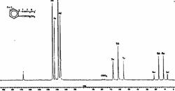
First we note the wide chemical shift range of the signals. Note also that the signal we attribute to the methyl group is approximately a 1:3:3:1 quartet, the methylene approximately a 1:2:1 triplet, and the aromatic CHs approximately 1:1 doublets. The intensity ratios suggest this is due to coupling and the multiplicities that it is due specifically to coupling of the spin 1/2 ¹³C with the spin 1/2 protons and nothing else (i.e. the 2nI+1 rule, I being the spin number). Before we move on to discuss how this coupling may be useful to us, let us remind ourselves of how the coupling arises. Remember the energy level diagram of one spin 1/2 nucleus in a magnetic field:

The precessing magnetisation vector either reinforces or opposes Bo, so that locally at least, other nuclei will perceive two slightly different values of Bo. Since the populations of each energy level are practically identical (equation 5), another nucleus close-by will resonate with equal probability at two slightly different Larmor frequencies (equation 1). The difference between these two frequencies is what we know at the coupling constant J. Its value depends on how the perturbation in Bo is transmitted between the two nuclei, and this is normally achieved via the intervening electrons (hence the term through bond coupling). When two identical nuclei are involved, three slightly different and equally spaced values of Bo, with the middle one being twice as probable as the highest or lowest, hence the 1:2:1 triplet coupling pattern we are familiar with. In spin terms, we say that four configurations are possible; +1/2,+1/2; +1/2, -1/2; -1/2, +1/2; -1/2, -1/2. As the middle two are of equal energy, this manifests as a double height peak, i.e. a 1:2:1 triplet. If we remember that J(coupling) = w_o/10⁶, these visible in the carbon spectrum above look in the range JC-H ~ 6 x 22 ~ 130 Hz. Notice that carbon appears not to couple with other carbons, only with protons in the same molecule. This is because the probability that two ¹³C-¹³C nuclei will be close enough to couple is 100 times less than the probability of finding ¹³C-¹²C as adjacent nuclei.

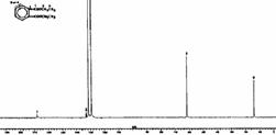
There are seven singlets; the spectrum is certainly less cluttered because the coupling has gone! It has been removed by a technique called broad band ¹H decoupling. During measurement of the ¹³C FID, the entire proton resonance region of the compound (i.e. from about -2 to + 10 ppm) was irradiated with "white noise" radio frequency. This has the effect of increasing the rate of transition between the proton low and high energy spin states such that only one average magnetic field is experienced by any individual carbon nucleus, and the manifestation of coupling vanishes. As far as the carbon is concerned all the protons cease to exist (well, almost. There is an effect called the nuclear Overhauser effect or nOe which does very odd things to the intensity of the carbon line, normally increasing it by a factor of two or more and hence is one of the factors making integration of ¹³C spectra unreliable.). Normally for ¹³C both decoupled and coupled spectra are recorded, but the latter with a small modification called "off-resonance proton decoupling";

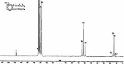
Here the proton decoupler is actually switched on during ¹³C measurement but its frequency is centred at about -10 ppm. It has the effect of removing any coupling between ¹³C and ¹H that occurs through more than one bond (H-C-C and longer range couplings of < 10Hz) but leaving coupling due to directly bonded atoms (i.e. H-C of >125 Hz) still visible (above). This reduces the complexity of the spectrum and offers a significant gain in the intensity of the signals (~ four fold reduction in measurement time) from the nOe enhancement referred to above.

Together, these two spectra give the following information:

· The proton decoupled spectrum tells the number of unique types of carbon atoms in the molecule (i.e. a mono-substituted phenyl group has four unique carbon atoms)

· The off-resonance spectrum tells how many hydrogen atoms are attached to each unique carbon (quartet=3, triplet=2, doublet =1, singlet = none).

· From the chemical shift of each carbon, much information about the environment of the carbon can be gleaned.

The typical chemical shift ranges of carbon nuclei are as follows:

C (alkane)	~ 0 - 30 ppm
C (alkene)	~ 110 - 150 ppm
C-N	~ 50
C-O	~ 60
C-F	~ 70 ppm.
Aromatic	~ 110 - 160 ppm
Ester, amide, acid,	~ 160-170 ppm
Ketone, aldehyde	~ 200-220 ppm.

Priors to sampling, of course, a pulse that nutate the magnetization in the XY plane, have been applied. The pulse and the receiver can be cycled together to get rid of some artefacts.

Empirical estimation of chemical shifts:

For paraffins the ¹³C chemical shift of the kth carbon can be represented by:

d (C_k) = B_s + N₃C_s + N₄D_s + M₂A_s2 + M₃A_s3 + M₄A_s4

s = number of carbon atoms bonded to the kth carbon; N₃ and N₄ are the numbers of carbon atoms 3 and 4 bonds away from the kth carbon; M₂, M₃, and M₄ are the numbers of carbon atoms bonded to the kth carbon and having 2,3,and 4 attached carbons respectively

B1	6.8	B2	15.34	B3	23.46	B4	27.77
C1	-2.99	C2	-2.69	C3	-2.07	C4	0.68
D1	0.49	D2	0.25	D3	0	D4	0
A12	9.56	A22	9.75	A32	6.60	A42	2.26
A13	17.83	A23	16.70	A33	11.14	A43	3.96
A14	25.49	A24	21.43	A34	14.70	A44	7.35

The effect of substituting a polar group in an alkane can be estimated from the substituent constants given by the following expression:

		d =-2.3+SZi+K+S
Z	Ca	Cb	Cg	Cd
H	0.0	0.0	0.0	0.0	Steric		S
C	9.1	9.4	-2.5	0.3	3p	A13	-1.1
Epoxide	21.4	2.8	-2.5	0.3	4p	A14	-3.4
-C=C-	19.5	6.9	-2.1	0.4	3s	A23	-2.5
Ethinil	4.4	5.6	-3.4	-0.6	4s	A24	-7.5
Ph	22.1	9.3	-2.6	0.3	2t	A32	-3.7
F	70.1	7.8	-6.8	0.0	3t	A33	-9.5
Cl	31.0	10.0	-5.1	-0.5	4t	A34	-15
Br	18.9	11.0	-3.8	-0.7	1q	A41	-1.5
I	-7.2	10.9	-1.5	-0.9	2q	A42	-8.4
O	49.0	10.1	-6.2	0.0	3q	A43	-15
-OCO-	56.5	6.5	-6.0	0.0	4q	A44	-25
-ONO-	54.3	6.1	-6.5	-0.5
-N	28.3	11.3	-5.1	0.0	Conformation
-N+	30.7	5.4	-7.2	-1.4	Dihedral		K
NO2	61.6	3.1	-4.6	-1.0		0°	-4
-NC	31.5	7.6	-3.0	0.0		60°	-1
-S-	10.6	11.4	-3.6	-0.4		120°	0
-SCO-	17.0	6.5	-3.1	0.0		180°	2
-SO-	31.1	9.0	-3.5	0.0		Free	0
-SO2Cl-	54.5	3.4	-3.0	0.0
-SCN	23.0	9.7	-3.0	0.0
-CHO	29.9	-0.6	-2.7	0.0
-CO-	22.5	3.0	-3.0	0.0
-COOH-	20.1	2.0	-2.8	0.0
-COO	24.5	3.5	-2.5	0.0
COO-	22.6	2.0	-2.8	0.0
-CON	22.0	2.6	-3.2	-0.4
-COCl	33.1	2.3	-3.6	0.0
-C=NOH sin	11.7	0.6	-1.8	0.0
-C=NOH anti	16.1	4.3	-1.5	0.0
-CN	3.1	2.4	-3.3	-0.5

C1: S=1; N3=2; N4=1; M2=1	d1= B1+2C1+D1+A12	d1= 6.8+2(-2.99)+0.49+9.56=10.87
C2: S=2; N3=1; N4=1; M3=1	d2= B2+C2+D2+A23	d2= 15.34+(-2.69)+0.25+16.7=29.6
C3: S=3; N3=1; N4=0; M2=2	d3= B3+C3+D3+A32	d3= 23.46+(-2.07)+2(6.6)=34.59
C4: S=2; N3=1; N4=0; M2=1;M3=1	d4= B2+C2+D2+A22+A23	d4= 15.34+(-2.69)+9.75+16.7=39.10
C5: S=2; N3=2; N4=1; M2=1	d5= B2+C2+D2+A22	d5= 15.34+(-2.69)+0.25+9.75=19.96
C6: S=1; N3=1; N4=1; M2=1	d6= B1+C1+D1+A12	d6= 6.8+(-2.99)+0.49+9.56=14.35
C7: S=1; N3=2; N4=1; M3=1	d7= B1+2C1+D1+A13	d7= 6.8+2(-2.99)+0.49+17.83=19.14

	Ca		Cb		Cc		Cd
Basic	-2.3	Basic	-2.3	Basic	-2.3	Basic	-2.3
a C	9.1	a C	9.1	3a C	27.3	a C	9.1
a COOH	20.1	b COOH	2.0	a -O-C=O	56.5	2b C	18.8
a NH	28.3	b NH	11.3	g NH	-5.1	b -O-C=O	6.5
b COO	2.0	g COO	-2.8	d C	0.3	d NH	0.0
d C	0.3
S(t,3)	-9.5	S(p,3)	-1.1	S(q,1)	-1.5	S(p,4)	-3.4
Calculated	48.0	Calculated	16.2	Calculated	75.2	Calculated	28.7
Reported	49.0	Reported	17.3	Reported	78.1	Reported	28.1

Isotope Effects on Chemical Shifts

Small changes in chemical shifts are often found on isotopic substitution. d ¹³C decreases by about 0.3 ppm on going from ¹³CHCl₃ to ¹³CDCl₃ (a "one-bond" effect), while d ¹⁹F decreases by 0.47 ppm in going from CH₂=CH₂ to CH₂=CD₂. Isotope effects are smaller in ¹H resonance, in keeping with the smaller total range of chemical shifts, d ¹H decreases by 0.019 ppm between CH₄ and CH₃D (a "two-bond" effect).

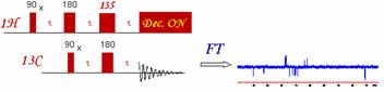
Enhancement of signals with polarization transfer via:

Insensitive Nuclei Enhanced by Polarization Transfer (INEPT)

(Also used for Multiplet Detection in Decoupled X-nuclei experiments)

The intensity of signals in NMR is governed by the magnetogyric ratio (g). This means that proton nuclei, which have a very high frequency, are the most sensitive nuclei. The population (at Boltzman equilibrium) is proportional to the g parameter. In the little graphic below, the larger proton population (in a spin state) is represented with larger dots, whereas the X nuclei with lower frequency (here Carbon-13) is represented with smaller dots.

The idea behind the INEPT pulse sequence is to selectively invert one of the proton transition in the doublet (from heteronuclei coupling) creating non equilibrium population in the AX spin system (to see this effect, just rollover the image below). Then after such selective inversion, the X nuclei can be observed with larger intensity. The enhancement ratio is: ± gH / gC (about 4 in the case of carbon).

Simple INEPT

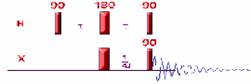
The first INEPT sequence published is a based on simple spin echo. As the first step in the pulse sequence is to apply a 90` pulse on proton nuclei, the relaxation delay that must be used in this experiment is based to proton relaxation rate (T₁(H))To see what's happening in this pulse sequence. A more complex rollover sequence, explaining what happen in each step of that pulse sequence can be found here

The double 180 degree pulse, applied to both nuclei in the middle of the evolution delay, refocus the chemical shift and field inhomogeneity but not the heteronuclear coupling constant which continue to dephase during the second evolution period. The evolution delay is adjusted such at the end of the 2*tau delay the doublet due to heteronuclei coupling has antiphase orientation (2*tau=1/2J). The last 90 degree pulse (applied to both nuclei) will simply selectively invert the population in one of the proton doublet component, polarizing thereby the population of the heteronuclei. The heteronuclei is therefore detected with an enhance intensity (gammaH/gammaX: gH / gC) that does not depends on the relaxation like the NOE enhancement)

Refocused INEPT

At the end of the normal INEPT sequence, the X-enhanced multiplet components are oriented anti-phase. Turning ON the decoupler at this moment would cancel the enhancement (as all antiphase multiplet components would now precess at the same frequency: chemical shift)!! The refocusing period in refocused INEPT will allow to reorient these components until they create additive effect. The optimum refocusing delay depends not only on the heteronuclear coupling constant JXH, but also on the number of protons n coupled to the heteronuclei.

If the refocusing delay is systematically varied, a 2DJ - INEPT spectra is obtained. To learn more about the INEPT,

DEPT (Distortionless Enhancement by Polarization Transfer)

The DEPT experiment is in fact an improved version of the INEPT experiment. It results also in an enhancement of the intensity of the X-nuclei by a factor of gH / gC. One of the nicest improvement of this sequence as compared with the INEPT, is that the DEPT experiment does not have to deal with a variable refocusing delay. Indeed, the magnetization from the X-nuclei multiplet is enhanced but "in phase" at the end of the pulse sequence. The intensity of the X nuclei is dependent on the length of the last proton pulse. Therefore, the DEPT experiment is less sensitive to a misset delay (but is very sensitive to proton pulse calibration). As the multiplet behavior of the X-nuclei is created by the last q proton pulse, coupled Carbon-13 spectra can be obtained with DEPT enhancement.

The starting point of the DEPT pulse sequence is, as we can see, a 90` pulse on proton. This means, the recycle delay is controlled (like in INEPT) by the proton relaxation rate. The tau delay t (1/2J) is chosen to maximize the antiphase components of the proton doublet but unlike INEPT, multiple quantum magnetization is created by the 90` pulse on the X heteronuclei. The second t delay serves as a refocusing period for proton chemical shifts.

The q proton pulse transforms the multiple quantum coherence into observable single quantum coherence. The 180` pulse applied to the X-nuclei ensures proper chemical shift on the X-nuclei. At the end of the third delay, the in-phase magnetization can then be detected (with the proton decoupler turned ON or OFF. The intensity of the X-nuclei signal depends on the length of the pulse controls and on the number of protons coupled to the X-nuclei.

· For singly protonated carbons - CH, the intensity of the signal can be calculated by: sin (q)

· For doubly protonated carbons - CH₂, the intensity of the signal can be calculated by: 2* sin (q) * cos (q)

· For triply protonated carbons - CH₃, the intensity of the signal can be calculated by: 4* sin (q) * cos² (q)

To distinguish the various multiplicity patterns in carbon-13 NMR, three DEPT spectra are acquired:

2D- Homonuclear Correlations COSY (COrrelated SpectroscopY).

Is one of the simplest and most useful experiment. It is also one of the shortest 2D experiment. It needs a minimum of 4 transients on conventional spectrometer (see phase cycling - vector model or coherence pathway). With the addition of gradients, only one transient is needed which means that on a modern spectrometer, the very precious COSY information can be obtained in 5 min!!!

This 2D experiment is composed of a 90 degree pulse that creates magnetization in the transverse plane. During the evolution time, the variable delay t1 is incremented systematically in order to sample the spectral width indirectly. Following this variable time period, a second pulse mixes the spin states, transferring magnetization between coupled spins. The spectrum is then acquired during t2 (detection time). After double Fourier Transformation, a spectrum like the one below is obtained showing a diagonal component (for magnetization that did not exchange magnetization) and cross peaks (off-diagonal) for nuclei exchanging magnetization through scalar coupling. The data is usually symmetrical respect to the diagonal and therefore the data can be symmetrized as part of the processing to improve the quality (care must be taken here to make sure that by getting rid of the non-symmetrical artefacts we are not also getting rid of precious information that might not be totally symmetrical). The data is usually acquired in a phase insensitive (magnitude mode) manner, avoiding the difficulty to phase a 2D data set. This phase insensitive mode gives rise to very broad lineshape that can be sharpen using sine-bell or pseudo-echo shaping processing method.

Phase sensitive COSY

If the COSY experiment is run in a phase sensitive fashion, the data result in a dispersive diagonal and antiphase absorptive cross-peak (up-down). The idea of running phase sensitive experiment is to be able to measure coupling constants directly from the 2D cross peaks (as in complex molecules severe overlapping prevent such measurement to be made). The dispersive nature of the diagonal peaks (broad tails) makes it very difficult to observe the COSY cross peaks close to the diagonal. Therefore other method should be used. For phase sensitive experiment, the DQF-COSY presents much better characteristics.

Double quantum filtered COSY (DQF-COSY)

Double quantum filtered COSY is a phase sensitive technique. This pulse sequence converts the dispersive diagonal peak into antiphase absorption (like the cross peaks). A minimum of 8 scans is required for the phase cycling but if gradients are used to select the coherence pathway, only one scan is needed. There are many variant of that phase sensitive COSY experiment (E-COSY, EZ-COSY ...) but they are all quite time consuming (these experiments can take up to 24 hours as they need to be run with sufficient resolution to extract couplings with good accuracy).

If the measure of coupling constant is needed, one of the best ways might be to use "soft-COSY". This soft experiment detects only the cross peak (antiphase absorption mode). As the spectral window is very narrow (only one multiplet in both dimensions), excellent resolution can be achieved in minutes! In soft COSY experiment, the first 90` pulse is replaced by a very selective pulse. The evolution time (t1) is then used to sample a very small window at F1 frequency. Then a selective pulse applied to 2 frequencies at the same time (the first selectively irradiated resonance and its coupled partner). This selective pulse will achieve the proper cross-peak selection. The detection at F2 will sample only the cross-peak.

Relay-COSY

The Relay-COSY experiment is a simple extension of the COSY experiment. It differs from COSY in the introduction of a refocusing period (tau-180-tau) followed by a second mixing pulse (90`). During the COSY part of the sequence (90-t1-90), if we have for example a three spin system AMX (where the A Nuclei is coupled only to M and the X nuclei is coupled only to M -> JAX=0), the A nuclei will exchange magnetization only with M; similarly, the X nuclei will exchange magnetization only with M. The purpose of the extra 2 tau delay is to allow some time for the COSY cross peak (AM or AX) to develop antiphase character respect to the coupling to another nuclei. Then the last 90` pulse mixes the spin states in such a way that even if A and X nuclei are not coupled together, there will be a cross peak between these two (mediated by the M nuclei which is coupled to both A and X). This sequence is very useful to provide information on the second neighbor in a complex spectrum.

In principle, this extra {tau-180-tau-90} part of the sequence can be repeated over and over again to provide multiple step relay-COSY. In practice, the longer relay-COSY experiments (relay2, relay3, relay4...) have very marginal usefulness: the 2*tau period is relatively long and for complex molecules, suffering usually from shorter relaxation rates, the magnetization have time to relax back to the Z axis, loosing the precious cross peak labeling.

NOESY (Nuclear Overhauser Enhanced SpectroscopY)

NOESY is one of the most useful techniques as it allows to correlate nuclei through space (distance smaller than 5Å). By measuring cross peak intensity, distance information can be extracted.

The pulse sequence starts as usual with a 90` pulse followed by an evolution time t1. This delay is varied systematically as usual to provide chemical shift information in the F1 domain. Then a 90` pulse transmit some of the magnetization to the Z axis and during the following mixing period, the non-equilibrium Z component will exchange magnetization through relaxation (dipole-dipole mechanism). This exchange of magnetization is known as NOE (Nuclear Overhauser Effect). After some time (shorter than the relaxation time T1), the transverse magnetization is restored and detected. If relaxation exchange (or chemical exchange) have taken place during the mixing time, cross peaks will be observed in the spectra.

The phase cycling ensure proper detection of NOESY signal. In small/medium size molecules, the mixing time can be selected to be about 80% of the relaxation time. For larger molecules, shorter mixing time should be used to avoid "spin-diffusion" problems.

In NOESY experiment, the distinction between cross peaks originating from NOE effect and those originating from chemical or conformational exchange is not easy. In small molecules, having long correlation time, the phase of the peak can be used as evidence:

· With Diagonal signal phased "up"

· NOE cross peak is phased "down"

· Chemical Exchange cross peak is phased "Up"

For large molecule, having short correlation time, the phase of the diagonal, the NOE cross peak and the exchange cross peak is the same. It is therefore impossible to distinguish NOE from chemical exchange. In this case, the ROESY (NOE in the rotating frame) pulse sequence should be used.

ROESY

The ROESY sequence is very similar to the NOESY in that it provides information concerning distance between nuclei. This technique is based on NOE in the Rotating Frame. This pulse sequence is almost identical as the one used for TOCSY. To avoid TOCSY artefacts, the power used to achieve spin-lock is reduced. Also to further reduce the chances of Hartmann-Hahn match, the Spin-Lock offset is shifted to one end of the spectra (instead of the center). The HOHAHA signals are very large compare to the ROE cross peaks. It is therefore essential to take as many precautions as necessary to cancel those signals. Also if HOHAHA peaks are present, relayed cross peaks can be observed (HOHAHA-ROESY or ROESY-HOHAHA).

Contrary to NOE that can be positive (for small molecule), negative (for large molecule) or null (if the correlation time happen to cancel the NOE), the ROE (NOE in the rotating frame) is always positive. Alternation in sign of the ROE effect allows to distinguish the "three-spin effect" from true small ROE).

The peak phase behavior from the ROESY experiment is as follows:

· If Diagonal peaks are phased "up" or positive

· ROE cross peaks will be phased "down" or negative

· HOHAHA peaks will be phased "up" or positive

· Exchange peaks will be phased "up" or positive

This experiment was called CAMELSPIN in earlier publications

2D: Heteronuclear: X-detected

The 2D experiments presented here are shift correlation experiments involving two different nuclei interacting with scalar coupling constant J_X-H. These experiments were very popular in the 80's but with the advance made in NMR, they have now been replaced by the highly sensitive reverse experiments which detects the highly sensitive protons instead of the low-gamma low-sensitivity X nuclei.

HETCOR (HETeronuclear COrrelation)

The HETCOR experiment is similar to the COSY experiment with the exception that it concerns two different nuclei. The simplest pulse sequence that can be proposed for such 2D involves simply two 90` pulses, the last one being applied simultaneously to both nuclei. The first pulse excites proton nuclei whose chemical shift is detected during the evolution period t1. The proton signal of interest is coupled not only to other protons but also to the heteronuclei (and therefore redoubled with a large coupling constant). The last proton pulse transfers proton magnetization to the X-nuclei (through scalar coupling) whose intensity will be modulated by the proton chemical shift. Of course, this experiment is not very useful as such as we would like to detect decoupled X nuclei at least!

The "real" HETCOR pulse sequence involves refocusing of the heteronuclei coupling during the evolution time (t1) by applying a 180 ` pulse to the X-nuclei so that the protons will retain only the homonuclear coupling constant. The next 1/2J delay insures an efficient signal intensity transfer to the X-nuclei by developing the antiphase character for the heteronuclear coupling. The simultaneous 90 degree pulses on proton and on the X-nuclei transfers the magnetization to the X-nuclei (antiphase components like in INEPT sequence) whose intensity is modulated by the proton chemical shift. The last delay allows for the X-antiphased components to refocus so that the proton decoupler can be turn on for the subsequent detection period (t2). As the X-nuclei can be coupled to 1, 2 or 3 protons, an "optimum" refocusing delay that takes into account the various multiplicities for the X-nuclei (doublet, triplet or quartet with INEPT enhancement) must be setup. The refocusing delay used in standard sequence is about 1/3J (good intensity on CH, CH2 and CH3 type of carbons). This INEPT based HETCOR have been used extensively in the past but is the sensitivity of this technique much lower if we compare with the reverse experiments (HMQC and HSQC).

HETCOR with proton decoupling

If the pulse sequence is modified to include a bird pulse in the middle on the evolution time (instead of an ordinary 180` pulse on the X-nuclei), the proton-proton coupling gets also decoupled resulting in higher sensitivity. In the BIRD sequence, the first proton 90` pulse stores the proton magnetization along the Z-axis. The net result of the BIRD sequence is that it inverts the labels of protons bound to C-12 while keeping intact the labels of the protons bound to C-13. This selective inversion will produce homonuclear decoupling at the end of the evolution period. The 180` pulse (applied to both nuclei) inverts the protons as well as the heteronuclear labels insuring also the refocus of the heteronuclei coupling. The last 90` pulse (of BIRD element) restores the proton magnetization, which continue to evolve for the second half of the evolution time. The proton magnetization is then transferred back using the usual INEPT transfer.

.

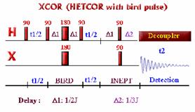These HETCOR and XCOR sequences can be further improved by including refocusing pulses in the INEPT transfer periods.

COLOC (COrrelated LOng range Coupling)

Modification of the delays in HETCOR can provide long range coupling information (coupling between proton and carbon through 2-3 bonds). The problem with these smaller heteronuclear couplings is that the pulse sequence gets dramatically longer, reducing the sensitivity of the experiment. An improvement to the HETCOR sequence is to make the evolution time constant and to include in it the INEPT polarization period (the net result is that the 180` pulse pair moves as a function of the evolution time such that at the end of the delay the proton magnetization coupled to the X-nuclei have acquired an antiphase character. Then, the INEPT polarization (double 90` pulse applied to both nuclei) can take place without further delay. This modification makes the pulse sequence shorter and more sensitive (less relaxation during the pulse sequence).

This sequence is quite insensitive and has been replaced by the inverse experiment: HMBC.

HETCOR-RELAY

This experiment combines the power of HETCOR with Relay-COSY. Although this experiment can be done by adding a "COSY-RELAY" step to the regular HETCOR sequence, the best way to do this experiment is by using a TOCSY mixing period after the HETCOR evolution period as shown in the figure below.

This pulse sequence is as sensitive as the HETCOR but again, with the evolution of NMR, these experiments are now best done in the inverse experiment mode (HMQC-TOCSY or HSQC-TOCSY).

2D-Heteronuclear: H-detected

HMQC (Heteronuclear Multiple Quantum Correlation)

The HMQC experiment provides correlation between protons and their attached heteronuclei through the heteronuclear scalar coupling. This sequence is very sensitive (compare to the older HETCOR) as it is based on proton detection (instead of the detection of the least sensitive low gamma heteronuclei).

The basic idea behind this experiment is in fact related to the echo difference technique, which is used to eliminate proton signals not coupled to the heteronuclei. (As a reminder, this cancellation is made possible by varying the phase of the pulses applied to the X nuclei (on alternate scans) and by subtracting the two signals - as can be seen in the figure below.

In this Spin Echo Difference experiment, a 180 degree (two 90` pulse with constructive phase: X, X) and no net pulse (two 90` pulse with destructive phase: X, -X) are applied on alternate scans. By subtracting the data in the receiver one cancel the unwanted protons attached to the unlabelled C-12. In order to get the 2D-shift correlation needed in HMQC, an evolution time t1 is introduced between the two heteronuclear 90` pulses.

· Therefore, the simplest version of the pulse sequence starts with a proton pulse followed by a 1/(2J) delay -During that delay, the proton magnetization (coupled to the heteronuclei) acquire anti-phase character.

· A 90` pulse applied to the X nuclei creates then multiple quantum magnetization which evolves under the influence of the X-chemical shift during the t1 evolution time (the proton chemical shift and heteronuclear coupling is refocused by using a 180` pulse at mid evolution time).

· At the end of the evolution period, another 90` pulse on the heteronuclei transfers the magnetization back into detectable (antiphase) single quantum proton magnetization, which is then left to evolve another 1/(2J) delay to refocus the antiphased magnetization.

· The alternation in the phase of the last 90` heteronuclei pulse with the alternation of the receiver phase provides cancellation of the unwanted proton not coupled to the X-heteronuclei.

· During the proton detection period, the X-nuclei coupling interactions can be decoupled using Waltz or Garp decoupling sequences.

The minimum phase cycling require 4 scans in the classical phase sensitive experiment. By using pulse field gradients to select the coherence, it is now possible to run this experiment with only one scan! - This means that with a modern spectrometer, 2D-Shift correlation involving proton and carbon can be obtained in 5 minute!

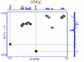
HSQC (Heteronuclear Single Quantum Correlation)

The HSQC experiment have been proposed by Bodenhausen and Ruben (G. Bodenhausen and D. J. Ruben, Chem. Phys. Lett., 69, 185 (1980)). The HSQC experiment is in fact a double INEPT experiment. This experiment correlates protons with their directly attached heteronuclei. Proton magnetization is detected (during t2 - detection time) while the low-gamma nuclei evolves during the evolution time - t1. Because of the detection of the high frequency nuclei, this sequence is very sensitive. The enhancement in sensitivity of this experiment is much greater than the enhancement obtainable by simple NOE (Nuclear Overhauser Effect). This is why this experiment has been referred to as the "OverBodenhausen" experiment.

· The HSQC experiment starts with proton magnetization. Therefore the recycle time is based on proton relaxation time (1.26 * T₁).

· The first INEPT step is used to create proton antiphase magnetization (2 tdelay) which is then transferred to the directly attached heteronuclei (Carbon, Nitrogen ...).

· This X nuclei magnetization is left to evolve with its chemical shift (during t1 - evolution time). The effect of proton coupling and chemical shift is removed by the use of a 180` proton pulse applied at mid evolution time.

· The double 90` pulse applied to both nuclei (in the beginning of the last INEPT step) transfers the magnetization back to proton as an anti-phased magnetization, which is then refocus during the last (2 tdelay). The proton in-phase magnetization can then be detected in the presence of the X-nuclei decoupler.

For further information, you can consult the literature for the comparison of the sensitivity of the HMQC and HSQC experiments.

A. Bax, M. Ikura, L.E. Kay, D.A. Torchia and R. Tschudin, J. Magn. Reson, 86, 304 (1990).

B. T.J. Norwood, J. Boyd, J.E. Heritage, N. Soffe and I.D. Campbell, J. Magn. Reson, 87, 488 (1990).

HMBC (Heteronuclear Multiple Bond Correlation)

The HMBC experiment detects long range coupling between proton and carbon (two or three bonds away) with great sensitivity. The length of the tau delay can be adjusted to detect relatively large coupling constants (4-10 Hz) tau = 0.06 s or smaller couplings (2-7 Hz) tau = 0.1 s.

In this sequence, the first 90` pulse on Carbon-13 serves as a low-pass filter that suppresses one-bond correlation and passes the smaller coupling. This pulse creates multiple quantum coherence for the one-bond coupling, which is removed from the spectra by alternating the phase of the Carbon-13 pulse. The second 90` pulse on C-13 creates multiple quantum coherence for the long-range couplings. After the evolution time t1, the magnetization is converted back into detectable single quantum proton magnetization. The carbon decoupler is never used in this sequence: therefore the protons displays homonuclear as well as heteronuclear couplings.

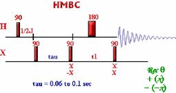
This technique is very valuable to detect indirectly quaternary carbons coupled to protons - especially useful if direct Carbon-13 is impossible to obtain due to low amount of material available. This very useful sequence provides information about the skeleton of a molecule. It could be an alternative to the 2D-INADEQUATE experiment (which is so insensitive). It is also very useful in carbohydrate area as a sequence analysis tool that provides unique information concerning connectivities across glycosidic linkages. Another area of interest for using HMBC is in the peptide-protein area - especially when applied to a ¹⁵N labeled protein - It is possible with this technique to get connectivities between the Nitrogen and the CH_a proton of the amino acid of the next residue^.

HMQC-TOCSY (HMQC combined with a TOCSY experiment)

This sequence combines the power of HMQC and TOCSY together. In this experiment the carbon (or other heteronuclei) chemical shift is detected first during the evolution time. The magnetization is then transferred to its directly attached proton, which is then correlated to the other protons in the same spin system during an MLEV mixing period prior to detection.

This experiment can be particularly useful in carbohydrate area as a tool that can spread the proton chemical shifts along the carbon axis. Indeed each carbon will correlate to its directly attached proton and to every proton that are part of the same sugar ring (the proton correlation depends on the length of the mixing period). Another application is in the peptide-protein area - when applied to ¹⁵N labeled protein - It is possible to get connectivities between the Nitrogen, the CH_a proton of the amino acid and the further away protons (depending on the length of the mixing time). The shift of the protons of each individual amino acid can be obtained that way (except for proline, which does not have NH proton).

There is also a version for HSQC-TOCSY.

HMQC-NOESY (HMQC combined with a NOESY experiment)

This sequence combines the power of HMQC and NOESY. In this experiment the carbon (or other heteronuclei) chemical shift is detected first during the evolution time. The magnetization is then transferred to its directly attached proton, which is then correlated to the other protons that are close in space prior to detection.

This technique have found application in the peptide-protein area - when applied to ¹⁵N labeled protein - It is possible to get connectivities between the Nitrogen, it's directly attached proton, and the protons that have NOE effect with it.

There is also a version for the HSQC-NOESY experiment.

References:

1) NMR Spectroscopy: Principles and Application, Six second year lectures given at Imperial College by Henry Rzepa. www.ch.ic.ac.uk/local/organic/nmr.html

2) The NMR facility at Queen's University, Sue Blake, www.chemqueensu.ca/PagWeb_RMN/Basic.HTM

3) L.M. Jackman and S. Sternhell, "Applications of NMR Spectroscopy in Organic Chemistry," 2nd ed., Pergamon Press, NY, 1969.

4) J.A. Feeney, S.M. Walker, J.A. Elvidge, P.W. Hickmott and O. Meth-Cohen, "Some Recent Developments in NMR Spectroscopy," in "An Introduction to Spectroscopic Methods for the Identification of Organic Compounds, "F. Scheinmann,Ed., Pergamon Press, NY, 1974, Vol.2.

5) R.J. Abraham and P. Loftus, "Proton and Carbon-13 NMR Spectroscopy, an Integrated Approach," Heyden & Son, Philadelphia, PA, 1978.

6) S.F. Dyke, A.J. Floyd, M. Sainsbury, and R.S. Theobald, "Organic Spectroscopy," 2nd ed., Longman, NY, 1978.

7) E.D. Becker, "High Resolution NMR: Theory and Chemical Applications," 2nd ed., Academic Press, NY, 1980.

8) G.C. Levy, R.L. Lichter, and G.L. Nelson, "Carbon-13 NMR Spectroscopy," 2nd ed., Wiley-Interscience, NY, 1980.

9) Atta-ur-Rahman, "Nuclear Magnetic Resonance: Basic Principles," Springer-Verlag, NY, 1986.

10) E. Derome, "Modern NMR Techniques for Chemistry Research," Pergamon Press, NY, 1987.

11) R.J. Abraham, J. Fisher, and P. Loftus, "Introduction to NMR Spectroscopy," 2nd ed., Wiley, NY, 1988.

12) Atta-Ur-Rahman, "One- and Two-Dimensional NMR Spectroscopy," Elsevier, NY, 1989.

13) R. M. Silverstein, G. C. Bassler and T. C. Morrill, Spectrometric Identification of Organic Compounds, 5th Ed., Wiley, 1991.

14) E. Pretsch, T. Clerc, J. Seibl y W. Simon, "Tablas para la Elucidación estructural de Compuestos Orgánicos por Métodos Espectroscópicos", Alhambra, Madrid, 1980.