SeriesFourierEjemplo.html

Series de Fourier de funciones pares o impares.

Onda cuadrada 1 (Per’odo T, intervalo (-T/2,T/2))

> restart:

> with(plots): setoptions(thickness=1):

Warning, the name changecoords has been redefined

> T:=2: Digits:=7:

Consideremos la siguiente funci—n onda cuadrada, de per’odo T, en el intervalo [ -T/2, t/2]

> f:=piecewise((-T/2<=t and t<0,-1),(0<=t and t<=T/2,1));
#latex(%);

> plot(f,t=-T/2..T/2);

> N:=20:t0:=-T/2: t1:=T/2:

Calculemos los coeficientes de Fourier y los coeficientes del espcctro de potencia

> for n from 0 to N do
a[n]:=2/T*int(f*cos(n*2*Pi/T*t),t=t0..t1):
b[n]:=2/T*int(f*sin(n*2*Pi/T*t),t=t0..t1):
A[n]:=sqrt(a[n]^2+b[n]^2):
phi[n]:=argument((b[n]+1E-10)+I*a[n]):
od:

Con ellos construimos la serie de Fourier

> SerieFourier := (m,t)->
                a[0]/2 +
                sum(a[k]*cos((2*k*Pi*t)/T),k=1..m) +
                sum(b[k]*sin((2*k*Pi*t)/T),k=1..m) ;

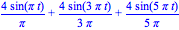
Verificamos algunas expansiones para n=5 y n=10

> SerieFourier(5,t);SerieFourier(10,t);

> plot([f,SerieFourier(3,t),SerieFourier(7,t), SerieFourier(20,t)],t=-T..T,title="Aproximaciones de Fourier: n=3 (Verde),n=7 (Azul), n=20 (negro) ",color=[red,green,blue,black],numpoints=100);
plot([f,SerieFourier(3,t),SerieFourier(7,t), SerieFourier(20,t)],t=-2*T..2*T,title="Aproximaciones de Fourier: n=3 (Verde),n=7 (Azul), n=20 (negro) ",color=[red,green,blue,black],numpoints=100);

> SeProm:=evalf(a[0]/2):

El espectro de potencia se puede graficar como

> Amp_a0:=plot([[0,0],[0,SeProm]],thickness=3 ):
Amp_coef:=[seq(plot([[n,0],[n,A[n]]]),n=1..N)]:
display(Amp_a0,Amp_coef,title=`Espectro de Potencia de la Se–al`);

Onda cuadrada 2

À quŽ hubiera pasado si el intervalo de integraci—n, o el per’odo hubiera sido diferente ?

Obvio que es la misma funci—n pero la contruimos de manera distinta. Consideremos la misma funci—n s—lo que diferente:

> restart:

> with(plots):

Warning, the name changecoords has been redefined

> T:=2: Digits:=7:

Consideremos la siguiente funci—n onda cuadrada, de per’odo T, en el intervalo [ -T/2, t/2]

> f:=piecewise((0 <=t and t<T/2,1),(T/2<=t and t<=T,-1));
#latex(%);

> plot(f,t=0..T);

> N:=20:t0:=0: t1:=T:

Calculemos los coeficientes de Fourier y los coeficientes espectrales

> for n from 0 to N do
a[n]:=2/T*int(f*cos(n*2*Pi/T*t),t=t0..t1):
b[n]:=2/T*int(f*sin(n*2*Pi/T*t),t=t0..t1):
A[n]:=sqrt(a[n]^2 + b[n]^2):
phi[n]:=argument((b[n]+1E-10)+I*a[n]):
od:

Con ellos construimos la serie de Fourier

> SerieFourier := (m,t)->
                a[0]/2 +
                sum(a[k]*cos((2*k*Pi*t)/T),k=1..m) +
                sum(b[k]*sin((2*k*Pi*t)/T),k=1..m) ;

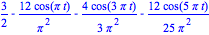
Verificamos algunas expansiones para n=5 y n=10

> SerieFourier(5,t);SerieFourier(10,t);

Como es la misma funci—n expresada en la base de Fourier, obviamente dan los mismos coeficientes. Con ello, la conclusi—n es que uno puede escoger a voluntad el intervalo (si es la misma funci—n) para que las integrales sean m‡s f‡ciles de evaluar.

claramente las gr‡ficas ser‡n las mismas.

> plot([f,SerieFourier(3,t),SerieFourier(7,t), SerieFourier(20,t)],t=-T..T,title="Aproximaciones de Fourier: n=3 (Verde),n=7 (Azul), n=20 (negro) ",color=[red,green,blue,black],numpoints=100);

plot([f,SerieFourier(3,t),SerieFourier(7,t), SerieFourier(20,t)],t=-3*T..3*T,title="Aproximaciones de Fourier: n=3 (Verde),n=7 (Azul), n=20 (negro) ",color=[red,green,blue,black],numpoints=100);

y el espectro de potencia, tambiŽn ser‡ el mismo....

> SeProm:=evalf(a[0]/2):

> Amp_a0:=plot([[0,0],[0,SeProm]],thickness=3):
Amp_coef:=[seq(plot([[n,0],[n,A[n]]]),n=1..N)]:
display(Amp_a0,Amp_coef,title=`Espectro de la Se–al`);

Diente de sierra 1 Intervalo [0,T]

Consideremos ahora la funci'on diente de sierra

> restart:

> with(plots): setoptions(thickness=2): assume(k,integer):

Warning, the name changecoords has been redefined

> T:=2: Digits:=7:t0:=0: t1:=T:

Esta funci'on viene descrita como

> f:=piecewise((t0<=t and t<t1,3*t));

> plot(f,t=t0..t1);

calculamos entonces los 20 primeros tŽrminos de la Serie de Fourier para esta funci—n.

> N:=20:

> for n from 0 to N do
a[n]:=2/T*int(f*cos(n*2*Pi/T*t),t=t0..t1):
b[n]:=2/T*int(f*sin(n*2*Pi/T*t),t=t0..t1):
A[n]:=sqrt(a[n]^2+b[n]^2):
phi[n]:=argument((b[n]+1E-10)+I*a[n]):
od:

anal'iticamente hubiera sido

> aa[0]:=2/TT*int(a*x,x=0..TT);

para el am—nico fundamental

> aa[k]:=2/TT*int(a*x*cos(k*2*Pi/TT*x),x=0..TT);

para los arm—nicos pares de orden superior y

> bb[k]:=2/TT*int(a*x*sin(k*2*Pi/TT*x),x=0..TT);#latex(%);

para la contribuci—n de los arm—nicos impares

> a[0],a[4],a[7],b[3],b[9];

Constrimos, entonces la serie de Fourier

> SerieFourier := (m,t)->
                a[0]/2 +
                sum(a[k]*cos((2*k*Pi*t)/T),k=1..m) +
                sum(b[k]*sin((2*k*Pi*t)/T),k=1..m) ;

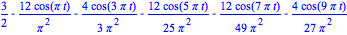
y evaluamos la serie para un par de desarrollos posibles n = 5 y n=10

> SerieFourier(5,t);#latex(%);
SerieFourier(10,t);

graficamos las representaciones de la funci—n para n=3, n=7 n=10

> plot([f,SerieFourier(3,t),SerieFourier(7,t), SerieFourier(10,t)],t=-T..T,title="Aproximaciones de Fourier: n=3 (Verde),n=7 (Azul), n=10 (negro) ",color=[red,green,blue,black],numpoints=100);

El promedio de la funci—n ser‡ la contribuci—n del arm—nico fundamental

> SeProm:=evalf(a[0]/2):

y esta ser‡ la contribuci—n del resto de los arm—nicos al espectro de potencia

> Amp_a0:=plot([[0,0],[0,SeProm]],thickness=3 ):
Amp_coef:=[seq(plot([[n,0],[n,A[n]]]),n=1..N)]:
display(Amp_a0,Amp_coef,title=`Espectro de la Se–al`);

Diente de sierra 2 (impar) Intervalo [-T/2,T/2]

> restart:

> with(plots): setoptions(thickness=2): assume(k,integer):

Warning, the name changecoords has been redefined

> T:=2:Digits:=7:t0:=-T/2: t1:=T/2:

> f:=piecewise((t0<=t and t<=t1,3*t));

> plot(f,t=t0..t1);

> N:=20:

> for i from 0 to N do
a[i]:=2/T*int(f*cos(i*2*Pi/T*t),t=t0..t1):
b[i]:=2/T*int(f*sin(i*2*Pi/T*t),t=t0..t1):
A[i]:=sqrt(a[i]^2+b[i]^2):
phi[i]:=argument((b[i]+1E-10)+I*a[i]):
od:

anal'iticamente hubiera sido

> aa[0]:=2/TT*int(a*x,x=-TT/2..TT/2);

para el am—nico fundamental

> aa[k]:=2/TT*int(a*x*cos(k*2*Pi/TT*x),x=-TT/2..TT/2);

para los arm—nicos pares de orden superior y

> bb[k]:=2/TT*int(a*x*sin(k*2*Pi/TT*x),x=-TT/2..TT/2);#latex(%);

> a[0],a[4],a[7],b[3],b[9];

> SerieFourier := (m,t)->
                a[0]/2 +
                sum(a[k]*cos((2*k*Pi*t)/T),k=1..m) +
                sum(b[k]*sin((2*k*Pi*t)/T),k=1..m) ;

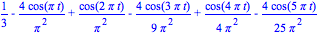
> SerieFourier(5,t); # latex(%);

> SerieFourier(10,t);

> plot([f,SerieFourier(3,t),SerieFourier(7,t), SerieFourier(20,t)],t=-T..T,title="Aproximaciones de Fourier: n=3 (Verde),n=7 (Azul), n=20 (negro) ",color=[red,green,blue,black],numpoints=100);

> SeProm:=evalf(a[0]/2):

> Amp_a0:=plot([[0,0],[0,SeProm]],thickness=3 ): Amp_coef:=[seq(plot([[n,0],[n,A[n]]]),n=1..N)]: display(Amp_a0,Amp_coef,title=`Espectro de la Se–al`);

Diente de Sierra 3 (par) Intervalo [-T/2,T/2]

> restart:

> with(plots): setoptions(thickness=2):

Warning, the name changecoords has been redefined

> T:=2: Digits:=7:t0:=-T/2: t1:=T/2:

> f:=piecewise((t0<=t and t<=0,-3*t),(0<t and t<=t1,3*t));

> plot(f,t=t0..t1);

> N:=20:

> for n from 0 to N do
a[n]:=2/T*int(f*cos(n*2*Pi/T*t),t=t0..t1):
b[n]:=2/T*int(f*sin(n*2*Pi/T*t),t=t0..t1):
A[n]:=sqrt(a[n]^2+b[n]^2):
phi[n]:=argument((b[n]+1E-10)+I*a[n]):
od:

anal'iticamente hubiera sido

> assume(k,integer):

> aa[0]:=2/TT*(int(-a*x,x=-TT/2..0) + int(a*x,x=0..TT/2));

para el am—nico fundamental

> aa[k]:=2/TT*(int(-a*x*cos(k*2*Pi/TT*x),x=-TT/2..0) +
int(a*x*cos(k*2*Pi/TT*x),x=0..TT/2));

para los arm—nicos pares de orden superior y

> bb[k]:=2/TT*(int(-a*x*sin(k*2*Pi/TT*x),x=-TT/2..0) +
int(a*x*sin(k*2*Pi/TT*x),x=0..TT/2));#latex(%);

> a[0],a[4],a[7],b[3],b[9];

> SerieFourier := (m,t)->
                a[0]/2 +
                sum(a[k]*cos((2*k*Pi*t)/T),k=1..m) +
                sum(b[k]*sin((2*k*Pi*t)/T),k=1..m) ;

> SerieFourier(5,t);#latex(%);

> SerieFourier(10,t);

> plot([f,SerieFourier(3,t),SerieFourier(7,t), SerieFourier(20,t)],t=-T..T,title="Aproximaciones de Fourier: n=3 (Verde),n=7 (Azul), n=20 (negro) ",color=[red,green,blue,black],numpoints=100);

> SeProm:=evalf(a[0]/2):

> Amp_a0:=plot([[0,0],[0,SeProm]],thickness=3 ):
Amp_coef:=[seq(plot([[n,0],[n,A[n]]]),n=1..N)]:
display(Amp_a0,Amp_coef,title=`Espectro de la Se–al`);

Par‡bola invertida

> restart:

> with(plots):

Warning, the name changecoords has been redefined

> T:=2: Digits:=7:t0:=-T/2: t1:=T/2:

> f:=piecewise((t0<=t and t<=t1,t^2));

> plot(f,t=t0..t1);

> N:=20:

> for n from 0 to N do
a[n]:=2/T*int(f*cos(n*2*Pi/T*t),t=t0..t1):
b[n]:=2/T*int(f*sin(n*2*Pi/T*t),t=t0..t1):
A[n]:=sqrt(a[n]^2+b[n]^2):
phi[n]:=argument((b[n]+1E-10)+I*a[n]):
od:

> SerieFourier := (m,t)->
                a[0]/2 +
                sum(a[k]*cos((2*k*Pi*t)/T),k=1..m) +
                sum(b[k]*sin((2*k*Pi*t)/T),k=1..m) ;

> SerieFourier(5,t);

> SerieFourier(10,t);

> plot([f,SerieFourier(3,t),SerieFourier(5,t), SerieFourier(10,t)],t=-T..T,title="Aproximaciones de Fourier: n=3 (Verde),n=7 (Azul), n=20 (negro) ",color=[red,green,blue,black],numpoints=100);
plot([f,SerieFourier(3,t),SerieFourier(5,t), SerieFourier(10,t)],t=-3*T..3*T,title="Aproximaciones de Fourier: n=3 (Verde),n=7 (Azul), n=20 (negro) ",color=[red,green,blue,black],numpoints=100);

> SeProm:=evalf(a[0]/2):

> Amp_a0:=plot([[0,0],[0,SeProm]],thickness=3 ): Amp_coef:=[seq(plot([[n,0],[n,A[n]]]),n=1..N)]: display(Amp_a0,Amp_coef,title=`Espectro de la Se–al`);

Una cuerda de longitud L

Sobre el eje x, consideremos una cuerda de longitud L fija en sus dos extremos. En x = xL/4 se desplaza y0. Encentre las expansiones en series de Fourier

> restart:

> with(plots):

Warning, the name changecoords has been redefined

> Digits:=7: L :=2: tp := L/4; y0:=L/10;

> f:=piecewise(( 0<=t and t<=tp,4*y0*t/L),
(tp<t and t<=L,(4*y0/3)*(-t/L +1)) );

> plot(f,t=0..L);

La serie con un per’odo L

> T:=L: t0:=0: t1:=L:

> N:=20:

> for n from 0 to N do
    a[n]:=2/T*int(f*cos(n*2*Pi/T*t),t=t0..t1):
    b[n]:=2/T*int(f*sin(n*2*Pi/T*t),t=t0..t1):
    A[n]:=sqrt(a[n]^2+b[n]^2):
    phi[n]:=argument((b[n]+1E-10)+I*a[n]):
od:

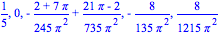
> a[0],a[4],a[7],b[3],b[9];

> SerieFourier := (m,t)->
                a[0]/2 +
                sum(a[k]*cos((2*k*Pi*t)/T),k=1..m) +
                sum(b[k]*sin((2*k*Pi*t)/T),k=1..m) ;

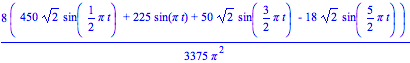
> SerieFourier(5,t);simplify(%);

> SerieFourier(10,t);simplify(%);

> plot([f,SerieFourier(3,t),SerieFourier(7,t), SerieFourier(10,t)],t=-T..T,title="Aproximaciones de Fourier: n=3 (Verde),n=7 (Azul), n=10 (negro) ",color=[red,green,blue,black],numpoints=100);

> SeProm:=evalf(a[0]/2):

> Amp_a0:=plot([[0,0],[0,SeProm]],thickness=3 ):
Amp_coef:=[seq(plot([[n,0],[n,A[n]]]),n=1..N)]:
display(Amp_a0,Amp_coef,title=`Espectro de la Se–al`);

La Serie antisimŽtrica respecto al eje x = 0 (per’odo 2 Lº)

> f:=piecewise( (-L <=t and t<-tp,(4*y0/3)*(-t/L -1)),
( -tp<=t and t<=tp,4*y0*t/L),
(tp<t and t<=L,(4*y0/3)*(-t/L +1)) );

> plot(f,t=-L..L);

> T:=2*L: t0:=-L: t1:=L:

> N:=20:

> for n from 0 to N do
a[n]:=2/T*int(f*cos(n*2*Pi/T*t),t=t0..t1):
b[n]:=2/T*int(f*sin(n*2*Pi/T*t),t=t0..t1):
A[n]:=sqrt(a[n]^2+b[n]^2):                                                     phi[n]:=argument((b[n]+1E-10)+I*a[n]):
od:

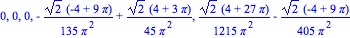
> a[0],a[4],a[7],b[3],b[9];

> SerieFourier := (m,t)->
                a[0]/2 +
                sum(a[k]*cos((2*k*Pi*t)/T),k=1..m) +
                sum(b[k]*sin((2*k*Pi*t)/T),k=1..m) ;

> SerieFourier(5,t);simplify(%);

> SerieFourier(10,t);simplify(%);

> plot([f,SerieFourier(3,t),SerieFourier(7,t), SerieFourier(10,t)],t=-T..T,y=-0.3..0.3,title="Aproximaciones de Fourier: n=3 (Verde),n=7 (Azul), n=10 (negro) ",color=[red,green,blue,black],numpoints=100);

> SeProm:=evalf(a[0]/2):

> Amp_a0:=plot([[0,0],[0,SeProm]],thickness=3):
Amp_coef:=[seq(plot([[n,0],[n,A[n]]]),n=1..N)]:
display(Amp_a0,Amp_coef,title=`Espectro de la Se–al`);

La Serie simŽtrica respecto al eje x = 0 (per’odo 2 Lº)

> f:=piecewise(         (-L <=t and t<-tp,(-4*y0/3)*(-t/L -1)),
                        ( -tp<=t and t<=0,-4*y0*t/L),
                        ( 0<t and t<=tp,4*y0*t/L),
                        (tp<t and t<=L,(4*y0/3)*(-t/L +1)) );

> plot(f,t=-L..L);

> T:=2*L: t0:=-L: t1:=L:

> N:=20:

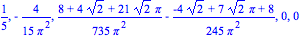
> a[0],a[4],a[7],b[3],b[9];

> SerieFourier := (m,t)->
                a[0]/2 +
                sum(a[k]*cos((2*k*Pi*t)/T),k=1..m) +
                sum(b[k]*sin((2*k*Pi*t)/T),k=1..m) ;

> SerieFourier(5,t):simplify(%);

> SerieFourier(10,t):simplify(%);

> plot([f,SerieFourier(3,t),SerieFourier(7,t), SerieFourier(10,t)],t=-T..T,y=-0.3..0.3,title="Aproximaciones de Fourier: n=3 (Verde),n=7 (Azul), n=20 (negro) ",color=[red,green,blue,black],numpoints=100);

> SeProm:=evalf(a[0]/2):

> Amp_a0:=plot([[0,0],[0,SeProm]],thickness=3 ):
Amp_coef:=[seq(plot([[n,0],[n,A[n]]]),n=1..N)]:
display(Amp_a0,Amp_coef,title=`Espectro de la Se–al`);

Onda cuadrada y Funci—n Teta de Heaviside

Consideremos la siguiente onda cuadrada

> restart;assume(n,integer):with(plots):
setoptions(thickness=2): # se hacen las lineas mas gruesas

Warning, the name changecoords has been redefined

> T :=2; y0 := 1;

> OndaCuad[0] := y0*(Heaviside(t)-Heaviside(t-T/2))
-y0*(Heaviside(t + T/2)-Heaviside(t));

> plot(OndaCuad[0],t=-2..2,y=-2..2,title="La Onda Cuadrada Basica");

> NT :=3:
for i from -NT to NT do
        tt := t - i*T;
        OndaCuad[i] := y0*(Heaviside(tt)-Heaviside(tt-T/2))
                        -y0*(Heaviside(tt +T/2)-Heaviside(tt));
end do:

> plot(sum(OndaCuad[j],j=-NT..NT),t=-4..4,y=-2..2,
title="La Onda Cuadrada de periodo L");

> f1 := -1;
f2 := 1;

El coeficiente y los coeficientes pares a[n] se anulan porque la funci'on es impar

> a[0]:=(2/T)*Int('f(t)',t=-T/2..T/2) = (2/T)*(int(f1,t=-T/2..0)+int(f2,t=0..T/2));A[0]:=rhs(%);

> a[n]:=(2/T)*Int('f(t)'*cos((2*n*t*Pi)/(T)),t=-T/2..T/2) = simplify((2/T)*(int(f1*cos((2*n*t*Pi)/(T)),t=-T/2..0)+int(f2*cos((2*n*t*Pi)/(T)),t=0..T/2)));

> A[k]:=subs(n=k,simplify((2/T)*(int(f1*cos((2*n*t*Pi)/(T)),t=-T/2..0)+int(f2*cos((2*n*t*Pi)/(T)),t=0..T/2))));

sobreviven los coeficientes impares

> b[n]:=(2/T)*Int('f(t)'*sin((2*n*t*Pi)/(T)),t=-T/2..T/2) = simplify((2/T)*(int(f1*sin((2*n*t*Pi)/(T)),t=-T/2..0)+int(f2*sin((2*n*t*Pi)/(T)),t=0..T/2)));

> B[k]:=subs(n=k,simplify((2/T)*(int(f1*sin((2*n*t*Pi)/(T)),t=-T/2..0)+int(f2*sin((2*n*t*Pi)/(T)),t=0..T/2))));

> SerieFourier := (m,t)->
                A[0]/2 +
                sum(A[k]*cos((2*k*Pi*t)/T),k=1..m) +
                sum(B[k]*sin((2*k*Pi*t)/T),k=1..m)         ;

> SerieFourier(5,t);

> SerieFourier(10,t);

> plot([OndaCuad[0],SerieFourier(3,t),SerieFourier(7,t), SerieFourier(20,t)],t=-1..1,title="Higher approximations: n=3 (Green),n=7 (Blue)",color=[red,green,blue,black],numpoints=100);